```{r}
#| label: example-chunk
#| warning: false
2+2
a <- "bob"
as.numeric(a)
```[1] 4
[1] NA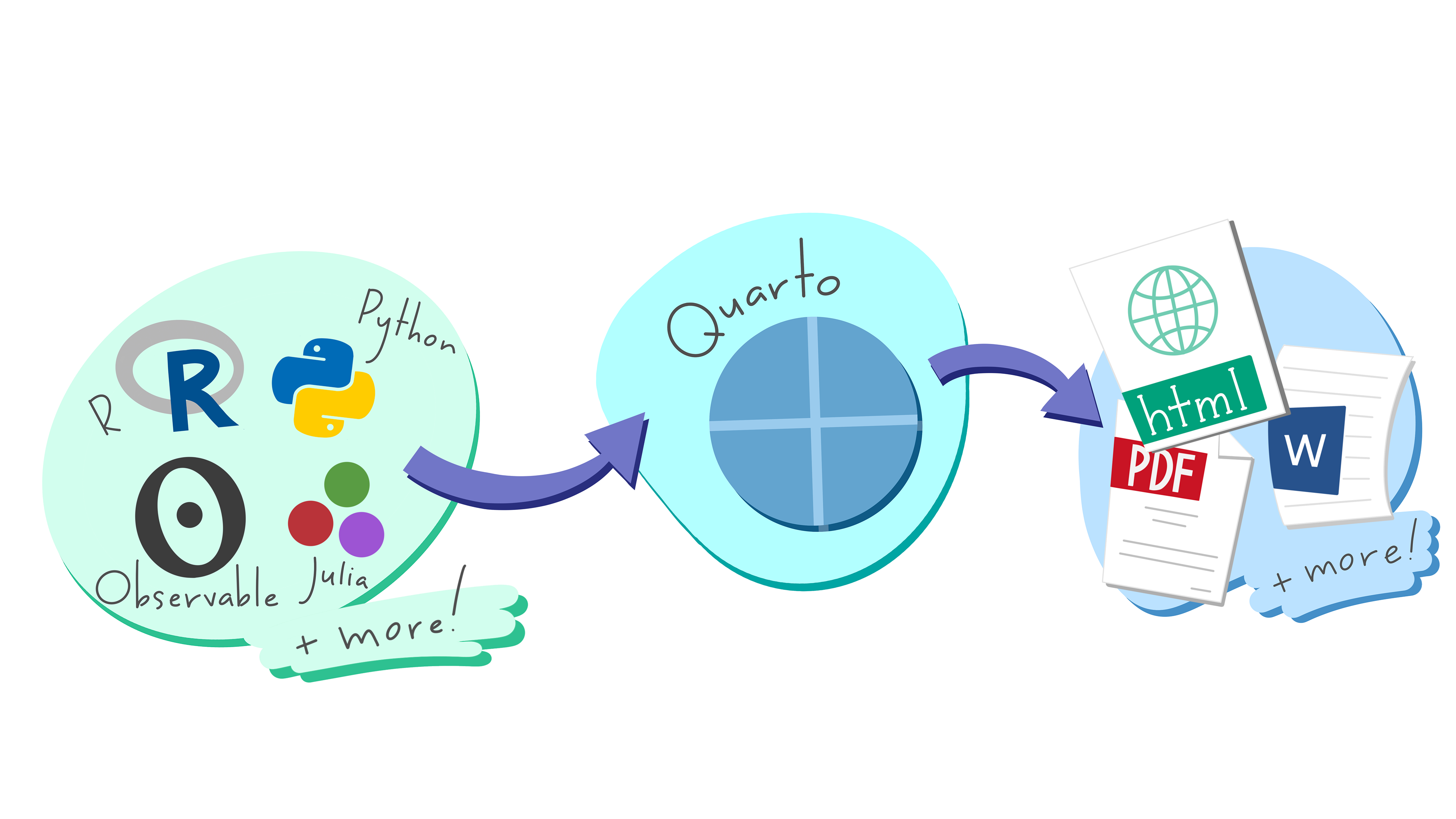
Quarto is a format for writing scientific and technical material in which bits of code from several different programming languages can be integrated into the written document. The document is then rendered to run the code and produce a final document in a variety of formats, including html, pdf, and Microsoft Word. The very textbook you are reading was produced in Quarto!
Quarto is also a second generation version of R Markdown. R Markdown does something similar but is only built to work with R. Quarto enables the user to include additional programming languages (like Python) as well into the final document and introduces a variety of other upgrades.
Quarto is also a form of reproducible report. A reproducible report uses some kind of automation to produce things like figures and tables. This has some advantages over the more traditional approach of transcribing results over to a final word processing document like Microsoft Word. First, transcription can introduce errors, both from typos and out-of-date results. When you automate the report, you can always be assured that you have the most up-to-date results without any transcription errors. Second, automating your output can ultimately save you a lot of time, because you won’t have to re-transcribe results when things change. You can just re-render the document and you are good to go.
You can use Quarto for a variety of things. The most obvious case is that you can write a full research manuscript, complete with automated citations. However, you can also use quarto documents instead of regular scripts for most tasks. In my own practice, I have begun using quarto documents rather than basic scripts for most things. These quarto documents then become a dynamic research log that both runs the analysis and reports on it. When you approach Quarto from this perspective, it eliminates the need for extensive commenting in your script because you can just write whatever you want.
Quarto itself is a command line program (like git) that is distinct from R and RStudio. However, it is fully integrated into RStudio (having been designed by the people at RStudio) so you generally won’t need to use the command line for much. You can download and install the most recent version of Quarto for your operating system here.
Once, you have Quarto installed, I would recommend two additional changes that will make working with Quarto easier. First, by default, Quarto will not be able to render to PDF documents because it needs an external latex program to do so (which I describe in more detail below). I highly recommend you use the tinytex latex package as it is lightweight and designed to work well with Quarto and R Markdown. To install it, you will need to use the command line. In RStudio, click on the “Terminal” tab next to console to get access to your command line. Then simply type:
quarto install tinytexYou can check that tinytex installed ok with:
quarto list toolsOccasionally, it will be necessary to update tinytex. To do so, simply type:
quarto update tinytexSecond, I recommend that you change your options in RStudio (through Tools > Global Options) in the following way. Go to the “R Markdown” options and change “Show output preview in” to “Viewer Pane.” This will make rendered output appear within RStudio rather than as an annoying pop-up window.
A quarto document is made up of three basic components:
Lets learn more about each of these components.
The document always begins with a header section that starts with a --- line and ends with the same line. A typical basic header might look like the example below.
---
title: A First Quarto Document
author:
  - Aaron Gullickson
  - Bob Coauthor
format:
  html:
    theme: litera
  pdf:
    toc: false
editor: visual
---
The format of this header is YAML which stands for YAML Ain’t Markup Language. The basi syntax of YAML is key: value. For example, the value of the key title in this case is “A First Quarto Document.” You do not have to surround values with quotes, although you may want to do so if the value contains special characters.
Keys can sometimes take multiple values, as is the case here for the author argument. You can specify multiple values by using a - to indicate each argument on a separate indented line.1
In some cases, arguments can have a nested structure, which can be indicated by indentation. In this case, I am specifying two different values for the format key which indicates what kind of document should be rendered. I have chosen both html and pdf. In each of those cases, I am specifying further keys that are specific to a given format. For example, the theme key specifies a particular theme for the html output.
The number of possible arguments you could provide is extensive. The guide at quarto.org provides a full list, but typically you can learn them on an as needed basis.
The YAML format can be very fussy. Its very common for starters to get errors in their yaml headers because of missing spaces or indentation. Be sure to indent with at least two spaces when necessary and leave a single space between the colon and the argument, or yaml will yell at you.
Most of your document will be written text, which is the hard part in the sense that you have to write the damn thing, but the easy part in terms of Quarto. All Quarto documents are plain text documents, just like basic scripts. You just write the text in the main body of your document. Paragraphs should be separated by an empty line. Do not indent paragraphs - Quarto will not recognize that as a new paragraph.
You can also add further markup to your text using the markdown language. A markup language provides a way to use syntax to represent how plain text should be displayed when rendered. The most well-known markup language is HTML, which is how web pages are encoded. Among geeky academics, the latex markup language has been used for decades to write technical documentation and research manuscripts. Compared to both of these examples, the markdown language is an absolute breeze. It is designed to be easy to learn and easy to read. The code block below introduces you to many of the basic elements of markdown.
#### Markdown Basics
What are some basic elements of markdown syntax? Well:
* I can put things in bullet point lists by starting with a `*` or a `-`.
* Indenting a bullet point by four spaces will create a sublist.
* Section headers can be indicated by starting the line with a sequence of `#`.
* The more `#` I provide, the deeper the subsection heading. e.g.,
* `#` is a top-level header.
* `##` is a second-level header.
* `###` is a third-level header.
* I can **bold** words by surrounding them with double asterisks `**`.
* I can *italicize* words by surrounding them with single asterisks `*`.
* I can create [links](https://google.com) with `[name](link address)`.
* I can create a footnote^[This is a footnote] with `^[footnote text].
* If I would rather have an numerated list, I can use numbers instead of `*`.
1. First
2. Second
3. Third
I can add an image with:

I can add blockquotes with:
> Four score and seven years ago our fathers brought forth on this continent, a
new nation, conceived in Liberty, and dedicated to the proposition that all men
are created equal.The markdown syntax is designed so that it doesn’t interfere with our ability to directly read the text. When this markdown text is rendered to a final document, it will look something like:
What are some basic elements of markdown syntax? Well:
* or a -.
#.
# I provide, the deeper the subsection heading. e.g.,
# is a top-level header.## is a second-level header.### is a third-level header, and so on.**.*.[name](link address).^[footnote text].*.
I can add an image with:

I can add a block quote with:
Four score and seven years ago our fathers brought forth on this continent, a new nation, conceived in Liberty, and dedicated to the proposition that all men are created equal.
The syntax above will usually be enough for academic manuscript writing, but if you want to try out markdown and learn other ways to use it, I recommend trying out this live markdown editor.
Code “chunks” are the big innovation of Quarto (and R Markdown before it). You can integrate code chunks into your document with the following syntax.
```{r}
#| label: example-chunk
#| warning: false

2+2
a <- "bob"
as.numeric(a)
```
[1] 4
[1] NATo start a code chunk, we begin with three “grave accents” (```) followed by curly brackets. Within the curly brackets, we indicate what programming language code will be within the code chunk. In this case, I want R code so I put “r”, but if you want python code, you could put “python”. The code chunk is closed by another sequence of three grave accents (```).
At the top of the code chunk, we can also include chunk options. The syntax for these chunk options is always3:
#| key: valueIn this case, I am specifying a label for the code chunk - it is good practice to label all of your code chunks. The second option is warning: false which indicates that any warnings produced by the code will not be shown in the output of the code chunk. In this case, trying to re-cast a character string into a numeric normally produces a warning message, but the warning message does not show up here in my output because I suppressed the warning.
You can see that the code chunk produced some basic output which is shown below the code chunk. This particular code chunk is not telling us anything useful, but the idea is that you can use code chunks to output important statistical results. As we will see below, we can also use it to produce beautiful figures and nice tables.
There are many chunk options that you can specify for a code chunk, but I want to focus on a couple that are useful. You have already seen warning but you may also want to set message: false to suppress messages that R may print when you run code.
You can also control whether the code is “echoed” in your rendered document. If you set echo: true then the code of the code chunk will be displayed along with the output in your final document. This can be useful for technical documentation, but if you are working on a final manuscript, you probably don’t want your code showing. In that case, you can set echo: false to hide the code and only show the output.mSimilarly, you can also hide your output with output: false.
If you want to set certain options as the default for all the code chunks in your document, you can specify this under the execute key in the YAML header. For example, if I wanted to turn off echo, message, and warning, I would add the following to my YAML header:
execute:
  echo: false
  warning: false
  message: false
I can still override these defaults in specific code chunks, but I don’t have to type in these defaults into every code chunk now.
You can run the code chunks in your document the same way you do from a script by using the run button or run hotkey on each individual line of code. Alternatively, you can run the entire code chunk interactively as shown in Figure 6.1. In either case, RStudio will give you an inline preview of the output in your document.
When writing code for your code chunks, remember that code chunks can use objects created by prior code chunks. Basically, R creates a whole new environment when you render the document so any code used in prior chunks will apply to further chunks.
When you run a code chunk in your document interactively, it will be able to access any objects that are currently loaded into your environment. However, when the final document is rendered, code chunks will be run from a new environment. This sometimes creates problems for students because their code chunk depends on an object (e.g. a dataset) that they loaded in some other way (e.g. by clicking on it in the files tab). The code works fine interactively, but when they try to render the document, they get an error about a missing object.
The solution to this problem is to ensure that any object you are referencing in your document is created or loaded in a prior code chunk within the document. Usually, I will start my documents with a “setup” code chunk that loads libraries and data to ensure I have what I need.
Ok, you finally have your first draft written and all of the code chunks are working. How do you render this Quarto document to a final product like a PDF or HTML file? As Figure 6.2 shows, its as easy as pushing the render button.

format in the YAML header. The actual rendered document will now be available in your working directory.
You will notice that before rendering the final document, R showed off a bunch of diagnostics as it built the file. Generally, you don’t have to worry about this, but it helps to know how Quarto gets from your original Quarto document to the final product.
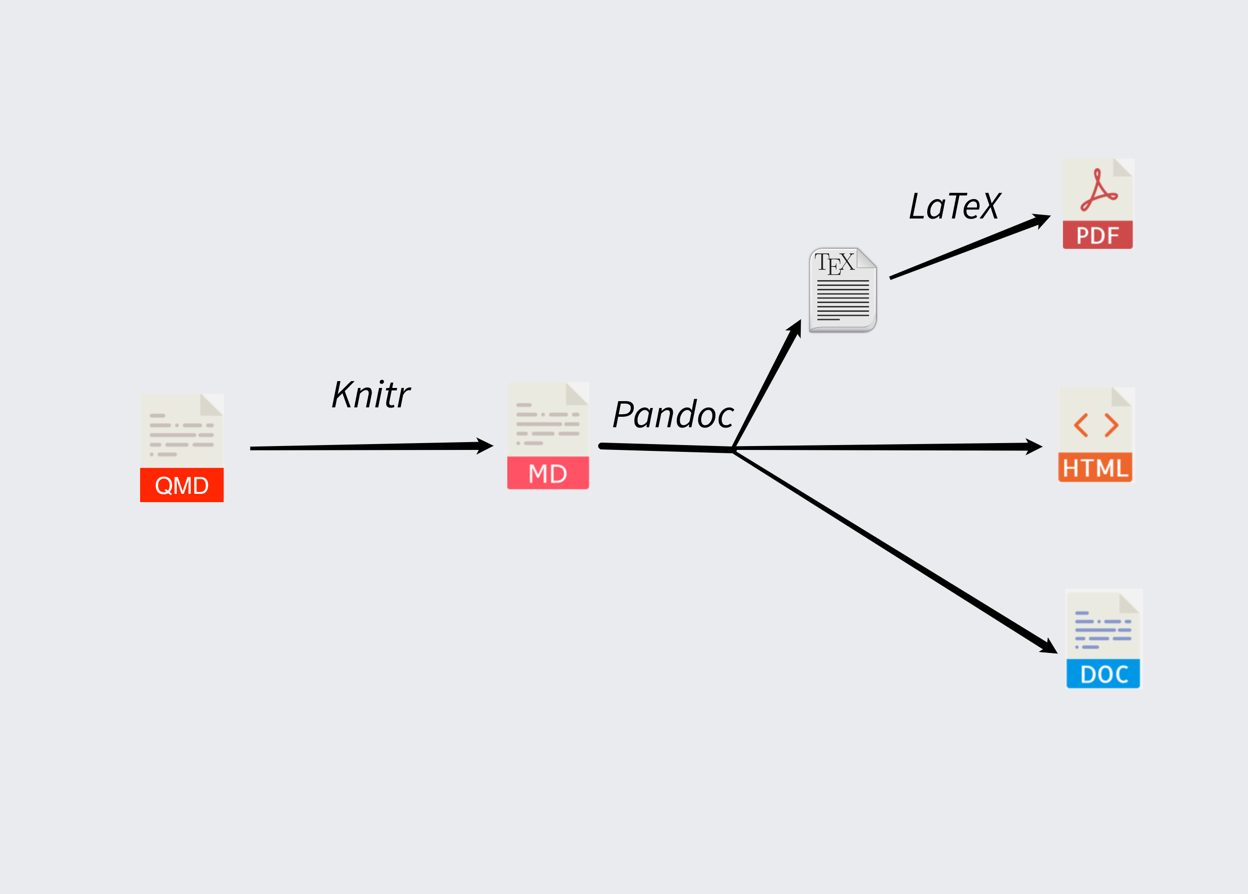
Figure 6.3 shows how this process works. The first step in the process is converting the Quarto documen to a basic markdown document. This is done by running the knitr library in R which executes all of the code chunks and replaces them with output and echoes where needed, as well as creating images for figures that are linked to the document.
Once your Quarto document has been transformed into a basic markdown document, the pandoc program converts it into another format. Pandoc is a standalone command line program that can convert to and from many different word processing and text formats. Pandoc is installed automatically with Quarto so you don’t have to worry about installing anything separately.
If you are rendering to HTML or a Microsoft Word document, Pandoc will directly convert the markdown file to that output type and you are done. Quarto will clean up any intermediate output produced in the process and your brand new shiny output format document will show up in your working directory.
If you are rending to PDF then a third step is necessary. You can’t go directly from markdown to PDF with Pandoc. Instead, Pandoc converts the markdown file to another markup language called LaTeX. LaTeX is a longstanding syntax used by academics and researchers to write technical documentation and manuscripts. Its not nearly as user friendly as Quarto, but does have an incredible flexibility.
To convert the LaTeX document to a final PDF document, you require a LaTeX engine. There are multiple engines to choose from, but the preferred engine for Quarto is TinyTex. If you followed my instructions above in when installing Quarto, you will already have a version of TinyTex installed and this part should go seamlessly. Otherwise, you will get an error about a missing LaTeX engine and will need to install one.c
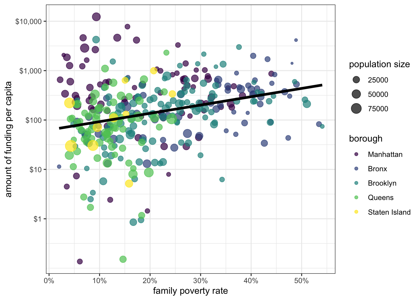
Quarto will beautifully display figures created from ggplot or other graphics packages. To add a figure to your Quarto document, you should write the code for that figure in a single code chunk that does nothing else. Additionally, your code chunk should contain at least the following chunk options:
fig-cap option that provides a caption for the figure. This is what we typically use to write captions for figures rather than the embedded titles in ggplot2.The code chunk below shows how to setup a code chunk to produce a nice figure, using the code from Chapter 5. Figure 6.4 shows what the output looks like.
```{r}
#| label: fig-nyc-final
#| fig-cap: Non-profit service funding to New York City health areas by poverty rate. Don't be afraid to add long captions to your figures to help readers understand them. Pictures are worth a thousand words, at least.
ggplot(nyc, aes(x=poverty, y=amtcapita))+
  geom_point(alpha=0.7, aes(color=borough, size=popn))+
  geom_smooth(method="lm", color="black", se=FALSE, size=1.5)+
  scale_x_continuous(label=scales::percent)+
    scale_y_log10(breaks=c(1, 10, 100, 1000, 10000),
                labels=scales::dollar(c(1, 10, 100, 1000, 10000)))+
  scale_color_viridis_d()+
  theme_bw()+
  labs(x="family poverty rate",
       y="amount of funding per capita",
       size="population size")
```
You can also cross-reference your figures in the main text of your document with @label where label is the label you used for the figure. This will apply the proper number to your figure and change it if you add more figures. This will only work if you started it with “fig-” so be sure to follow that syntax.
When you render your document to a PDF format, figures may “float.” They may not appear in the document exactly where you placed them in the text. Because a PDF document has to fit on a page, LaTeX will float figures to a nice place typically at the top or bottom of a page so that the text is not broken up. If you have a lot of figures relative to text, your figures may all end up floating to the back of your document. Just remember to not refer to your figures by “the figure below” but by properly cross-referencing them.
Adding nice tables in Quarto is a bit trickier than figures because tables vary enormously in their style and layout. If you want to display a pre-built tibble as a simple table in a Quarto document, you can use the kable command from the knitr package, as shown in the code chunk below and Table 6.1.
```{r}
#| label: tbl-movie-summary
#| tbl-cap: Summary statistics for movies by genre.
movies |>
  group_by(genre) |>
  summarize(n = n(),
            mean_runtime = round(mean(runtime), 1),
            mean_box_office= round(mean(box_office), 1),
            mean_metascore= round(mean(metascore), 1),
            percent_r=round(100*mean(maturity_rating=="R"), 1)) |>
  knitr::kable(col.names=c("genre",
                           "n",
                           "mean runtime",
                           "mean box office returns",
                           "mean metascore",
                           "percent R-rated"))
```| genre | n | mean runtime | mean box office returns | mean metascore | percent R-rated |
|---|---|---|---|---|---|
| Action | 411 | 114.6 | 62.7 | 51.4 | 56.0 |
| Animation | 240 | 94.2 | 113.1 | 56.8 | 2.9 |
| Biography | 358 | 116.7 | 26.7 | 61.8 | 50.3 |
| Comedy | 1182 | 101.5 | 34.8 | 50.3 | 50.3 |
| Drama | 301 | 109.2 | 11.3 | 59.6 | 66.1 |
| Family | 230 | 104.0 | 69.0 | 47.7 | 0.0 |
| Horror | 413 | 98.6 | 33.1 | 45.3 | 69.5 |
| Musical | 163 | 108.1 | 25.3 | 54.8 | 41.7 |
| Mystery | 78 | 111.2 | 20.7 | 59.3 | 70.5 |
| Romance | 230 | 111.2 | 17.3 | 56.1 | 53.9 |
| Sci-Fi/Fantasy | 442 | 113.9 | 100.4 | 50.0 | 23.3 |
| Sport | 50 | 112.3 | 20.0 | 55.0 | 28.0 |
| Thriller | 219 | 110.5 | 28.8 | 55.5 | 79.9 |
| Western | 26 | 113.8 | 27.2 | 61.4 | 69.2 |
You can see from the code chunk above that we use chunk options similar to figures for tables. I define a label that starts with “tbl-” which I can use to cross-reference the table in the text. I also provide a tbl-cap for a caption to the table.
The knitr::kable command can be good for basic tables, but does not provide a great deal of customization options for more complex tables. If you need a more complicated table, the best option is the gt package, which tries to apply a “grammar” to tables in a way analogous to ggplot2. The code chunk below uses gt package to create Table 6.2.
```{r}
#| label: tbl-movie-summary-gt
#| tbl-cap: Summary statistics for movies by genre.
movies |>
  group_by(genre) |>
  summarize(n = n(),
            mean_runtime = mean(runtime),
            mean_box_office= mean(box_office),
            mean_metascore= mean(metascore),
            prop_r=mean(maturity_rating=="R")) |>
  gt() |>
  cols_label(mean_runtime = "runtime",
             mean_box_office = "box office returns",
             mean_metascore = "metascore",
             prop_r="R-rated") |>
  cols_align("left", genre) |>
  tab_spanner("mean value", 3:5) %>%
  fmt_number(columns=c(mean_runtime, mean_metascore), decimals = 1) |>
  fmt_currency(mean_box_office, decimals = 0, scale_by = 1000000) |>
  fmt_percent(prop_r, decimals = 1) |>
  tab_source_note(md("*Source*: Internet Movies Database (IMDB) 2000-2021, supplemented with data from the Open Movie Database."))  |>
  tab_options(quarto.disable_processing = TRUE)
```| genre | n | mean value | R-rated | ||
|---|---|---|---|---|---|
| runtime | box office returns | metascore | |||
| Action | 411 | 114.6 | $62,696,594 | 51.4 | 56.0% |
| Animation | 240 | 94.2 | $113,147,083 | 56.8 | 2.9% |
| Biography | 358 | 116.7 | $26,671,229 | 61.8 | 50.3% |
| Comedy | 1182 | 101.5 | $34,838,917 | 50.3 | 50.3% |
| Drama | 301 | 109.2 | $11,330,233 | 59.6 | 66.1% |
| Family | 230 | 104.0 | $68,981,739 | 47.7 | 0.0% |
| Horror | 413 | 98.6 | $33,061,985 | 45.3 | 69.5% |
| Musical | 163 | 108.1 | $25,341,718 | 54.8 | 41.7% |
| Mystery | 78 | 111.2 | $20,721,795 | 59.3 | 70.5% |
| Romance | 230 | 111.2 | $17,314,783 | 56.1 | 53.9% |
| Sci-Fi/Fantasy | 442 | 113.9 | $100,425,792 | 50.0 | 23.3% |
| Sport | 50 | 112.3 | $19,970,000 | 55.0 | 28.0% |
| Thriller | 219 | 110.5 | $28,847,032 | 55.5 | 79.9% |
| Western | 26 | 113.8 | $27,203,846 | 61.4 | 69.2% |
| Source: Internet Movies Database (IMDB) 2000-2021, supplemented with data from the Open Movie Database. | |||||
Creating the table starts with feeding a tibble or data.frame into the gt command. We then pipe the output through a series of additional commands that modify parts of the table or add new parts. These commands are organized into groups identified by the name before the underscore.
Because tables can be so diverse, the number of possible functions in gt is extensive and too much to cover here, but let me briefly describe what the commands are doing to create this specific table. First, the cols_labels commands applies better column headers for the dataset than the R variable names. Second, cols_align aligns the text column for genre which would be otherwise centered. Third, the tab_spanner inserts a label directly above the three columns in the middle to group them together.
Most of the remaining commands are fmt_ commands that can be used to format the cells of particular columns. I use this to better display the percentages in the “R-rated” column and the dollar amounts in the box office returns column. I also use it to round values for the remaining two mean columns. Note that when using knitr::kable in the previous code chunk, I had to do all of this rounding and formatting before feeding the tibble into knitr::kable. In gt, this preliminary work is not necessary because it can all be done with the fmt_ commands.
Finally, I add a note to the table with tab_source_note. I wrap the text of this note in an md command which allows me to use markdown syntax (in this case, to italicize Source:).4
Just as with ggplot2, the best approach to gt is to start with a simple table and build in more features as needed to get it looking right. You can discover all kinds of additional formatting tools at the gt package website.
You may have noticed that the document I rendered in Figure 6.1 had citations and references. These citations are also automated and connected to a Zotero bibliography. Whenever the document is rendered, the citations are updated and a reference list is added to the end of the document.
To make use of this system, you will need to have a Zotero bibliography. I recommend
You can also specify multiple values with the syntax [Aaron Gullickson, Bob Coauthor]↩︎
This is a footnote↩︎
Technically, the use of the # sign here works because that is the comment symbol for R. If you are using a programming language with a different comment symbol, you should replace that with the appropriate commenting symbol followed by the pipe (|).↩︎
The one remaining command is necessary for Quarto to not apply some additional formatting to the table that I don’t want here, like striping.↩︎