So far, we have been speaking as if your research project only has one raw data source. You load this raw data source, recode variables, clean it up, and save the analytical dataset. In practice, many research projects will pull from multiple raw data sources. In some cases, these data sources may lead to multiple analytical datasets. However, in many cases, you will need to ultimately merge these datasets into a single analytical dataset.
As an example, lets take the world bank data that we have been working with for the last few chapters. In the code chunk below, I am using all the tricks of the trade we have learned to read this data into R and format it as the kind of tidy analytical dataset we want.
world_bank <-read_csv("data/world_bank.csv", n_max =651, na ="..", skip =1, col_names =c("country_name", "country_code", "series_name", "series_code","year2018", "year2019")) |># drop series_nameselect(!series_name) |># rename values of series_codemutate(series_code =case_when( series_code =="NY.GDP.MKTP.CD"~"gdp_capita", series_code =="SP.DYN.LE00.IN"~"life_exp", series_code =="EN.ATM.CO2E.PC"~"carbon_emissions")) |># pivot into longest format possiblepivot_longer(cols =c(year2018, year2019), names_to ="year", names_prefix ="year") |># recast year as numericmutate(year =as.numeric(year)) |># pivot wider into country-year formatpivot_wider(names_from = series_code,values_from = value)world_bank
# A tibble: 434 × 6
   country_name   country_code  year    gdp_capita life_exp carbon_emissions
   <chr>          <chr>        <dbl>         <dbl>    <dbl>            <dbl>
 1 Afghanistan    AFG           2018  18053222735.     63.1            0.299
 2 Afghanistan    AFG           2019  18799444415.     63.6            0.298
 3 Albania        ALB           2018  15156424015.     79.2            1.85
 4 Albania        ALB           2019  15401826127.     79.3            1.75
 5 Algeria        DZA           2018 174910684782.     76.1            3.92
 6 Algeria        DZA           2019 171760275467.     76.5            3.99
 7 American Samoa ASM           2018    639000000      NA             NA
 8 American Samoa ASM           2019    647000000      NA             NA
 9 Andorra        AND           2018   3218418632.     NA              6.59
10 Andorra        AND           2019   3155150256.     NA              6.29
# ℹ 424 more rows
The world bank data is a great resource for cross-national data. However, if you are trying to put together a cross-national dataset, you may find other data sources that you would like to combine with this world bank data. A prime example is the Varieties of Democracy (VDEM) data which provides a variety of democracy indices for countries over time. In this case, I want to include the VDEM score for liberal democracy v2x_libdem in my final country dataset.
To get started, let me load up the VDEM data, which I downloaded as a CSV file.1
vdem <-read_csv("data/vdem/V-Dem-CY-Full+Others-v13.csv.gz") |>select(country_name, country_text_id, year, v2x_libdem) |>filter(year ==2018| year ==2019)vdem
# A tibble: 358 × 4
   country_name country_text_id  year v2x_libdem
   <chr>        <chr>           <dbl>      <dbl>
 1 Mexico       MEX              2018      0.448
 2 Mexico       MEX              2019      0.433
 3 Suriname     SUR              2018      0.624
 4 Suriname     SUR              2019      0.593
 5 Sweden       SWE              2018      0.885
 6 Sweden       SWE              2019      0.875
 7 Switzerland  CHE              2018      0.872
 8 Switzerland  CHE              2019      0.87
 9 Ghana        GHA              2018      0.63
10 Ghana        GHA              2019      0.614
# ℹ 348 more rows
The goal is to merge this VDEM data into my World Bank data to make the liberal democracy variable a part of that overall dataset. You can already see that we have some other variables that will ideally let us identify the same country and year across datasets. Examining that is where we need to start.
Checking Your Keys
In order to merge two datasets, we need to have some id variables that are shared across the datasets which we call keys. In some cases, this may be a single variable with a numeric or alphanumeric id. In other cases, we need multiple keys to properly identify observations. In this case, we need both a country identifier and a year identifier.
The year part is easy. Both datasets have a year variable recorded as a numeric value. We can match years across datasets on this variable without problem. However, the country identifier is much trickier. An obvious candidate would be country_name, but as we will learn below this is a bad option because country names are often not consistent across data sources. We also have a three letter code called country_code in the world bank data and country_text_id in the VDEM data. This seems more promising.
However, before we proceed with trying to merge on these characteristics, we need to check our keys. Just like other parts of our data wrangling process, checking ourselves is a very important step when merging datasets. In this case, we want to understand whether our keys really are comparable across the two datasets. You might even want to ask yourself the question:
Yes, it turns out that you are both the gatekeeper and the keymaster! So lets vet some keys.
Lets start by thinking through the numbers here. We have two years of data from the VDEM and 358 observations, so that means we have 179 total countries in the VDEM dataset. Similarly, in the World Bank data, there are 434 observations over 2 years, so we have 217 countries. These results suggest that the VDEM dataset has slightly less coverage than the World Bank data. However, we can’t assume from this comparison that all of the countries in the VDEM dataset are wholly contained within the World Bank data.
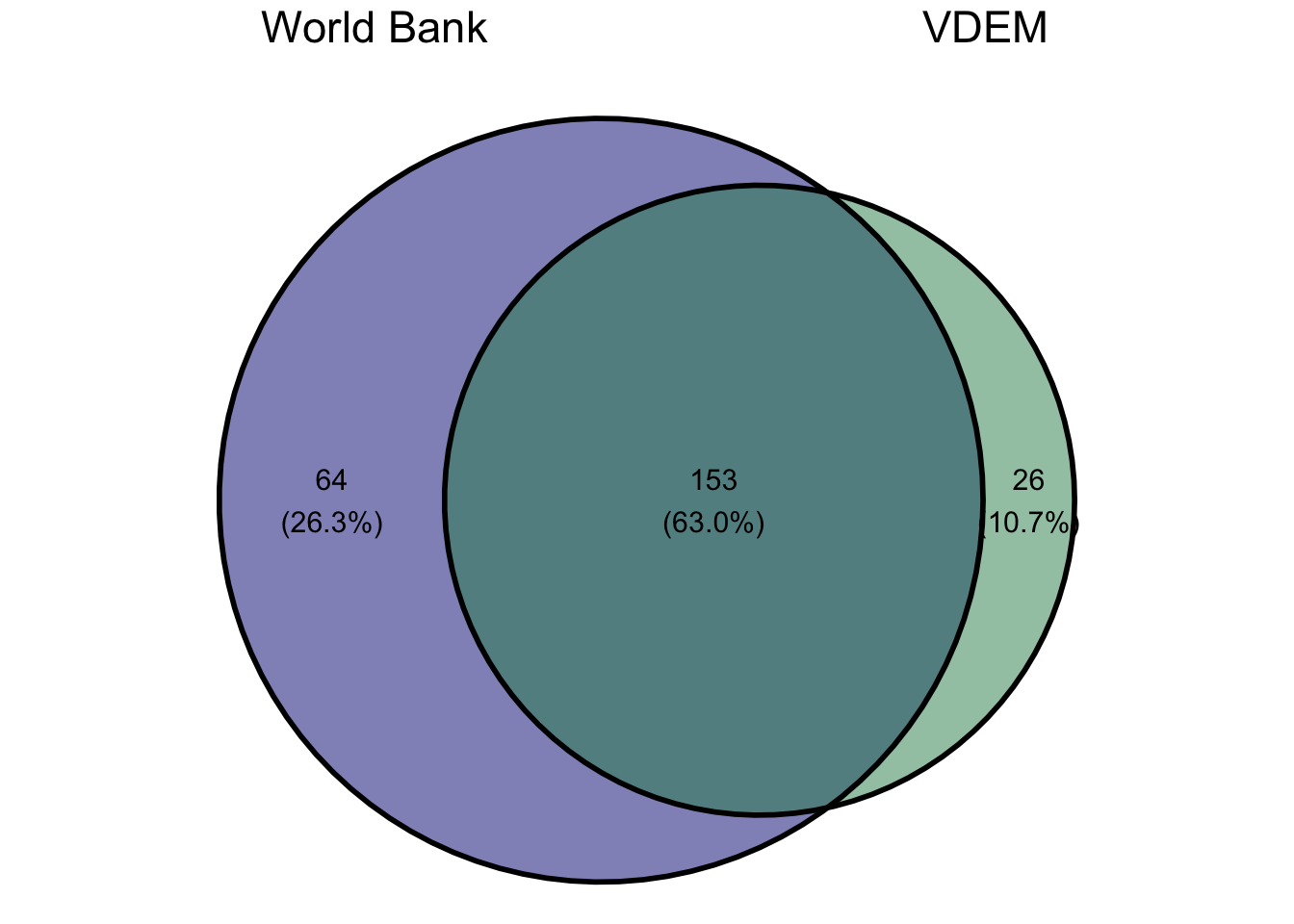
One way to first check our keys is to visualize overlaps using a Venn diagram. We can do this using the ggvenn R library. We feed into the ggvenn function a list, where each element of the list is a character vector of the unique country names from each data source. The ggvenn function will then figure out the overlaps and produce a Venn diagram as shown in Figure 11.1.
Figure 11.1: Venn diagram showing correspondence between country names in the world Bank and VDEM datasets. While there is substantial overlap, both datasets contain quite a few country names not found in the other dataset.
As you can see from Figure 11.1, we have many country names that do not find a match in the other dataset for both datasets. The World bank dataset contains 64 country names that are not matched in the VDEM dataset. We expected to see at least 38 cases like this because the World Bank has 38 more countries than the VDEM data. However, number of missing countries is substantially larger than 38, suggesting a problem.
We also have 26 cases in the VDEM data that are not found in the World Bank data. This is even more concerning because we generally expect the World Bank data to have better scope and thus expect the VDEM countries to be wholly contained within the World Bank data.2 Overall, the results suggest that our key of country name has some problems.
To explore this further lets identify more specifically these non-matching cases in both datasets. To do this we are going to make use of the %in% operator in R. The %in% operator will tell you if a value or set of values are contained within another vector of values. So for example, we could do something like:
# is bob in the list of names?"bob"%in%c("bob", "sally", "jim")
[1] TRUE
# is mike in the list of names?"mike"%in%c("bob", "sally", "jim")
[1] FALSE
# are bob and mike in the list of names?c("bob", "mike") %in%c("bob", "sally", "jim")
[1] TRUE FALSE
# are bob and mike not in the list of names?!(c("bob", "mike") %in%c("bob", "sally", "jim"))
[1] FALSE TRUE
In this case, we can make use of this operator to identify which country names from one dataset are not in the country names for the other dataset. Because, each country name is duplicated exactly twice by year, we also feed the results here through a unique function to just get unique unmatched values.
Lets use this approach to first look at the 64 country names from the World Bank that we did not find in VDEM.
Looking through the list, we can see that there are quite a few micro-nations (e.g. Faroe Islands, Liechtenstein, Monaco) and small island nations. Its understandable why these small countries may not be in the VDEM. However, we are also missing some alarming cases like the Russian Federation, both North and South Korea, Turkey (notably spelled “Turkiye) and the … United States. Something clearly is not right here.
To help solve this mystery, lets take a look at the 26 country names from VDEM that found no counterpart in the World Bank data.
 [1] "Burma/Myanmar"                    "Russia"
 [3] "Egypt"                            "Yemen"
 [5] "United States of America"         "Vietnam"
 [7] "North Korea"                      "South Korea"
 [9] "Taiwan"                           "Venezuela"
[11] "Ivory Coast"                      "Cape Verde"
[13] "Iran"                             "Syria"
[15] "Turkey"                           "Democratic Republic of the Congo"
[17] "Republic of the Congo"            "The Gambia"
[19] "Kyrgyzstan"                       "Laos"
[21] "Palestine/West Bank"              "Palestine/Gaza"
[23] "Somaliland"                       "Hong Kong"
[25] "Slovakia"                         "Zanzibar"
Looking through this list, you might see some familiar names. For example, this list contains the “United States of America.” Why didn’t we find a match for this case? Because in the World Bank data, the country name is just listed as “United States.” Similarly, in this list we have “Turkey” while in the other list we have “Turkiye.”
The problem here is that country names are not a reliable key. Country names are not consistent. Formal country names (“The Democratic People’s Republic of Korea”) may differ from colloquial usage (“North Korea”) and even colloquial terms may depend on language choice (“Turkey” vs “Turkiye”). We need a key that is more reliable.
Thankfully, we have a more reliable key in the form of the three letter country codes. These country codes are based on country ISO codes developed by the International Organization for Standardization. They are intended to be applicable across countries regardless of the actual country name used. These codes should provide a more reliable key for matching the two datasets.
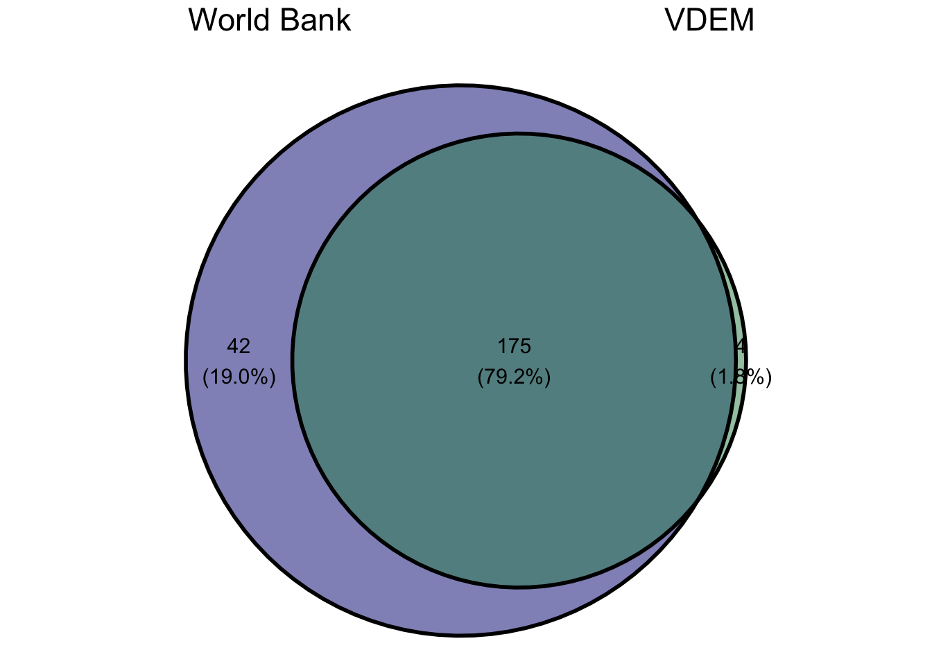
Figure 11.2: Venn diagram showing correspondence between country codes in the world Bank and VDEM datasets. The VDEM data is almost wholly contained within the World Bank data but we do have four cases of VDEM data not found in the World Bank data.
Figure 11.2 shows a Venn diagram of how these country codes overlap. We can see that the VDEM data is almost wholly contained within the World Bank data which is promising. However, we do have four country codes in the VDEM data that are not present in the World Bank data. Lets look more closely at these four cases:
These four cases all have something in common. They are either areas whose nationality is contested or semi-autonomous areas within larger nations. The World Bank data leaves all such cases out of its data (likely for political reasons). So, these four missing cases make sense.
We can also check on cases that are included with the World Bank data but missing from the VDEM data.
These are all small or micro-nations and thus it is unsurprising that the VDEM has not developed scores for them. Importantly, we don’t see any of the four countries listed above as missing from the World Bank masquerading here under another name.
In short, we are now satisfied that the country codes in each dataset will correctly identify matches across the two datasets. The only countries we will lose are ones that are not shared across the two datasets. Excellent work, keymaster!
Joining the Datasets
To merge cases, we are going to use the *_join functions available in the dplyr package. There are four *_join functions, but they all have the same basic arguments and functionality. In all cases, the first two arguments to the function are the datasets that you want to merge. Where the functions differ is in how they handle unmatched cases:
full_join
In this case, all unmatched cases in both datasets will be included with missing values for all variables in the unmatched dataset. Noting the sizes in Figure 11.2, I can see that this will result in a final merged dataset of 221 countries.
inner_join
In this case, all unmatched cases in both datasets are dropped. In essence, we only return the intersection of the Venn diagram in Figure 11.2, giving us the 175 countries where we had data from both sources.
left_join
In this case, all unmatched cases in the first dataset argument (the “left” dataset) are retained and all unmatched cases in the second dataset are dropped. If I feed in the World Bank data first, this option will retain all of the countries from the World Bank, but they will have NA values on the liberal democracy variable from VDEM.
right_join
This case is identical to left_join except that we retain all of the unmatched cases in the second dataset entered (the “right” one) and drop all the unmatched cases in the first dataset. The primary reason we have both a left and right join option is so that we can do joining more easily through a pipe.
Deciding which join you want depends on the research context. In this case, I only want one variable from VDEM, and the remainder of my variables are coming from the World Bank. Since all of these World Bank variables will be missing, it really makes no sense to keep the unmatched VDEM data. However, it may make sense to keep the World Bank data even when VDEM is missing, because I can still do lots of analysis without the liberal democracy variable, or I could use some kind of imputation to deal with missing values on that case. For that reason, I am going to use a left_join here.
When we merge datasets, the join function will look for variables with identical names across the two datasets and treat all of these variables as matching keys. In our case, that will be a problem because the three letter codes are named differently in the two data sources, but country_name which we don’t want to match on is the same across the two datasets. Therefore, if we just do:
left_join(world_bank, vdem)
We will end up matching on country_name and not the three letter ISO code. To correct this issue, we can specify a by argument that lists more specifically what variable names we want to match on. In this case, because the names are different across datasets, we have to feed into this argument a join_by function that gives a more complex syntax of how to relate key names across the two datasets, by using key_d1 == key_d2 for all keys we want to match on, separated by commas:
left_join(world_bank, vdem, by =join_by(country_code == country_text_id, year == year))
# A tibble: 434 × 8
   country_name.x country_code  year    gdp_capita life_exp carbon_emissions
   <chr>          <chr>        <dbl>         <dbl>    <dbl>            <dbl>
 1 Afghanistan    AFG           2018  18053222735.     63.1            0.299
 2 Afghanistan    AFG           2019  18799444415.     63.6            0.298
 3 Albania        ALB           2018  15156424015.     79.2            1.85
 4 Albania        ALB           2019  15401826127.     79.3            1.75
 5 Algeria        DZA           2018 174910684782.     76.1            3.92
 6 Algeria        DZA           2019 171760275467.     76.5            3.99
 7 American Samoa ASM           2018    639000000      NA             NA
 8 American Samoa ASM           2019    647000000      NA             NA
 9 Andorra        AND           2018   3218418632.     NA              6.59
10 Andorra        AND           2019   3155150256.     NA              6.29
# ℹ 424 more rows
# ℹ 2 more variables: country_name.y <chr>, v2x_libdem <dbl>
You can see that the merging appeared to work. Furthermore because we used a left_join the sample size of the World Bank data was preserved in this merged dataset. However, you might also notice that we now have two country_name variables: country_name.x and country_name.y. This is because both datasets contained a variable of this exact name but we explicitly did not match on this variable. Therefore, to retain these variables in the final merged data, the join function adds a suffix to each. the “.x” suffix indicates the first dataset (World Bank) and the “.y” suffix indicates the second dataset (VDEM).3
This is understandable, but I also don’t really like having this variable bloat in my final merged dataset. I really only need one country name variable, and since I am keeping all of the World Bank data, it makes more sense to use those country names in the final merged data.
We can more effectively (and easily) use the join command if we do a little preparatory work on the datasets we want to merge prior to joining. In this case, I want to do two things:
Remove country_name from the VDEM dataset.
Rename country_text_id from the VDEM dataset as country_code.
# A tibble: 358 × 3
   country_code  year v2x_libdem
   <chr>        <dbl>      <dbl>
 1 MEX           2018      0.448
 2 MEX           2019      0.433
 3 SUR           2018      0.624
 4 SUR           2019      0.593
 5 SWE           2018      0.885
 6 SWE           2019      0.875
 7 CHE           2018      0.872
 8 CHE           2019      0.87
 9 GHA           2018      0.63
10 GHA           2019      0.614
# ℹ 348 more rows
These simple steps will make my join much simpler because now the only variable names that match across the two datasets are exactly the keys that I want to use. So, to merge these datasets, I can use a much simpler left_join:
combined <-left_join(world_bank, vdem)combined
# A tibble: 434 × 7
   country_name   country_code  year    gdp_capita life_exp carbon_emissions
   <chr>          <chr>        <dbl>         <dbl>    <dbl>            <dbl>
 1 Afghanistan    AFG           2018  18053222735.     63.1            0.299
 2 Afghanistan    AFG           2019  18799444415.     63.6            0.298
 3 Albania        ALB           2018  15156424015.     79.2            1.85
 4 Albania        ALB           2019  15401826127.     79.3            1.75
 5 Algeria        DZA           2018 174910684782.     76.1            3.92
 6 Algeria        DZA           2019 171760275467.     76.5            3.99
 7 American Samoa ASM           2018    639000000      NA             NA
 8 American Samoa ASM           2019    647000000      NA             NA
 9 Andorra        AND           2018   3218418632.     NA              6.59
10 Andorra        AND           2019   3155150256.     NA              6.29
# ℹ 424 more rows
# ℹ 1 more variable: v2x_libdem <dbl>
I now have a combined dataset that retains all of my World Bank data and simply adds the liberal democracy score (where available) as another measure to that dataset.
In general, like other data wrangling operations, merging datasets requires good checks on your part to ensure you are not mismatching or missing potential matches. Additionally, you can save yourself a lot of headaches when joining by organizing your datasets prior to the join so that the only shared variable names across the two datasets are for keys that you want to use in the join.
I additionally gzipped this file to make it smaller.↩︎
You may also note that 64-26 equals 38 which is the difference in size between the two datasets. Mathematically this always has to be true.↩︎
You can also control what the suffix is with the suffix argument. I could for example have specified suffix=c("wb","vdem") to get something more intuitive.↩︎