Data doesn’t always come to us in the form that we need it to be for analysis. I am not speaking here of just the values and types of the variables it contains, but the actual form or shape of the data. In many cases, we may need to reshape the data to meet our needs.
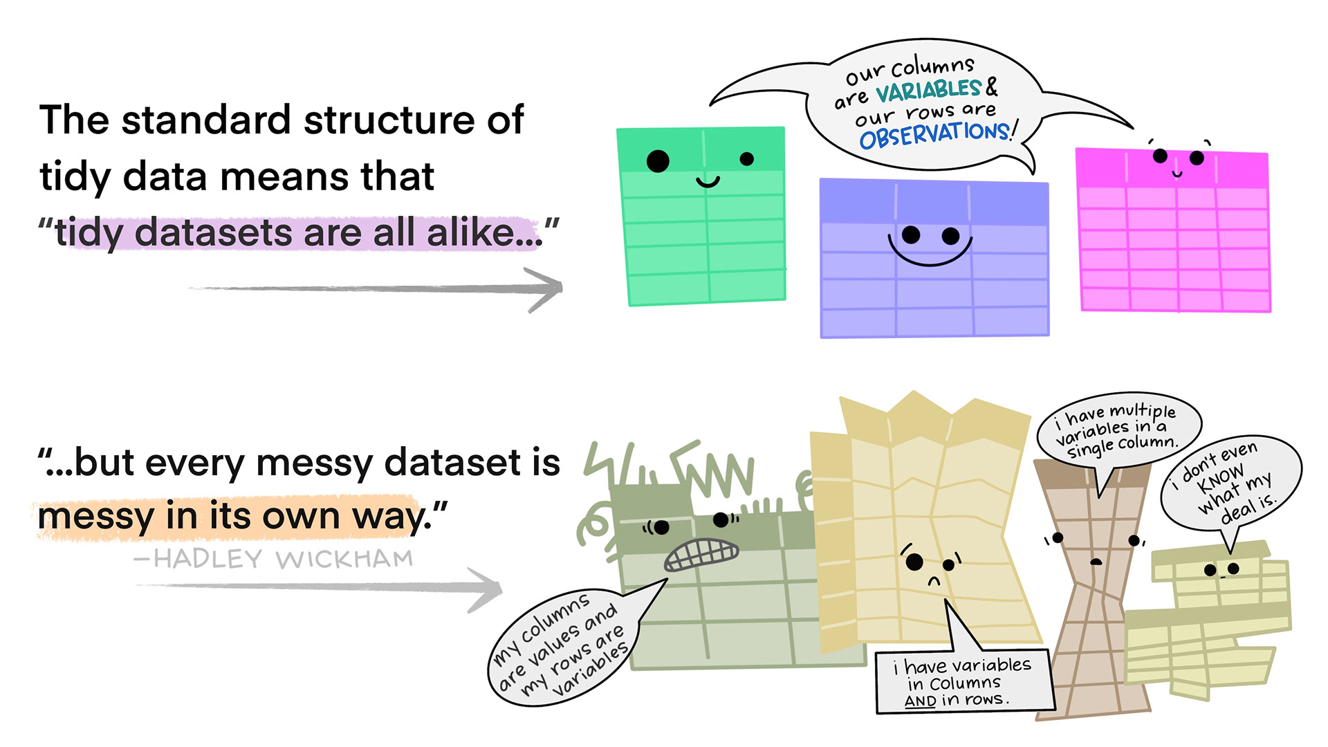
In particular, I am interested in two kinds of reshaping that we may need to do the original dataset. First, the data might not come to us in a tidy format and we may need to reshape it to comply with a tidy format. What do I mean by a tidy format? According to Hadley Wickham, a tidy dataset should conform to the following rules:
Each variable is a column; each column is a variable.
Each observation is a row; each row is an observation.
Each value is a cell; each cell is a single value.
This is generally the “spreadsheet” view of data that I have been using in this book. However, data is sometimes not distributed in this format, as we will see in the examples below. We may need to reshape such data into the desired format.
Furthermore, sometimes the distinction between observations and variables can be fuzzy. This is particularly true with data where you have repeat observations on units over time. Lets say I have yearly observations on countries. Should this data be organized so that an observation is a country and I have separate variables on the same measurement by year (e.g. gdp2018, gdp2019, etc.)? This is called a wide format and might look something like Table 10.1.
Table 10.1: Country data organized in a wide format. Each observation is a country.
Country
gdp2018
gdp2019
gdp2020
life_exp2018
life_exp2019
life_exp2020
Afghanistan
…
…
…
…
…
…
Albania
…
…
…
…
…
…
Belarus
…
…
…
…
…
…
Alternatively, I could organize the data by unique country-year observations. In this case, I will have separate variables to identify country and year and only single values for each measurement (e.g. just gdp). This long format data will look something like Table 10.2.
Table 10.2: Country data organized in a long format. Each observation is a country-year.
Country
year
gdp
life_exp
Afghanistan
2018
…
…
Afghanistan
2019
…
…
Afghanistan
2020
…
…
Albania
2018
…
…
Albania
2019
…
…
Albania
2020
…
…
Belarus
2018
…
…
Belarus
2019
…
…
Belarus
2020
…
…
These kinds of issues can be resolved by learning how to reshape data from wide to long formats and vice-versa. The pivot_wider and pivot_longer functions from the tidyr package will allow us to do this.
Another kind of reshaping is the case of aggregation. In this case, the data you have are on the wrong unit of analysis. Your data will have a nested structure such that lower-level units are nested within higher-level units. For example, you might have individual workers nested within organizations, or you might have individual students nested within classrooms which are nested within schools. You might want to calculate summary statistics like means and proportions at one of the higher levels of nesting. For example, you might want to know mean wages and years of education of workers by organization. Or you might want to know mean test scores of students and racial composition of schools.
In both of these cases, you want to aggregate the data from a lower unit of analysis to a higher unit of analysis. We can do this in R using the group_by and summarize functions.
Reshaping Wide and Long
To better understand the need for reshaping, lets take a look again at the world bank data we read into R in Chapter 7.
# A tibble: 651 × 6
   country_name   country_code series_name         series_code year2018 year2019
   <chr>          <chr>        <chr>               <chr>          <dbl>    <dbl>
 1 Afghanistan    AFG          GDP (current US$)   NY.GDP.MKT… 1.81e+10 1.88e+10
 2 Afghanistan    AFG          Life expectancy at… SP.DYN.LE0… 6.31e+ 1 6.36e+ 1
 3 Afghanistan    AFG          CO2 emissions (met… EN.ATM.CO2… 2.99e- 1 2.98e- 1
 4 Albania        ALB          GDP (current US$)   NY.GDP.MKT… 1.52e+10 1.54e+10
 5 Albania        ALB          Life expectancy at… SP.DYN.LE0… 7.92e+ 1 7.93e+ 1
 6 Albania        ALB          CO2 emissions (met… EN.ATM.CO2… 1.85e+ 0 1.75e+ 0
 7 Algeria        DZA          GDP (current US$)   NY.GDP.MKT… 1.75e+11 1.72e+11
 8 Algeria        DZA          Life expectancy at… SP.DYN.LE0… 7.61e+ 1 7.65e+ 1
 9 Algeria        DZA          CO2 emissions (met… EN.ATM.CO2… 3.92e+ 0 3.99e+ 0
10 American Samoa ASM          GDP (current US$)   NY.GDP.MKT… 6.39e+ 8 6.47e+ 8
# ℹ 641 more rows
The data is supposed to contain information by country on GDP per capita, life expectancy, and CO2 emissions for the years 2018 and 2019. However, take a close look at the data. What does one row of this data represent? Its not a single country because we have three lines of data for each country. However, its not a country-year either because we have year specific variables. There is only one way to describe this dataset:
We are mad1 scientists, though, so we can still make it work. Lets first figure out whats going on. If you take a close look what you will realize is that the multiple rows for each country represent the different variables, as indicated by the series_name and series_code variables. The variables of year2018 and year2019 thus record measurements on different variables in the same year. On line 1, we have GDP per capita for Afghanistan. On line 2, we have life expectancy at birth in Afghanistan. On line 3, we have CO2 emissions for Afghanistan. In its current form, the dataset is so bizarrely structured that it is useless. However, the tidyr::pivot_ commands will allow us to make it useful.
Its best to start by thinking how we do want this data to be structured. We can choose either a long or a wide format. In a long format, each row will be a country-year observation and will look something like Table 10.2 above.
However, because of the unusual structure of this dataset, regardless of how I want the ultimate data, I will need to reshape the dataset as long as possible first in order to reshape it into the ultimate forme that I want. Before I get started, it will help to do some prepatory work. I don’t need the series_name variable, so I am dropping that. Furthermore, I want to use more intuitive labels for the values of the series_code variable than what is showing. Because these names will ultimately become variable names, I am going to use the kind of syntax I want for variable names.
Notice that while I use to have three observations per country, I now have six observations per country. That is because I am not representing year as a variable with two values (for 2018 and 2019). All the actual values of the variables are represented in the value column.
How did pivot_longer do that. The only required argument for pivot_longer is cols. Here I specify columns that I want to be combined in a longer format. The variable names will then be represented by a names column and their value will be represented by a values column. The remaining variables will just be duplicated across all observations. Notice that I also used names_prefix to remove the word “year” from the front of each variable.
In this case, I used the names_to column to indicate an alternative column name for the names column. I now have this data as long as it can possibly be where each country is indexed by both a variable and year column and all values are recorded in a single values column. From this state, I can now reshape it wider to either a more traditional country-year long format or a country wide format.
Before I do that I want to make one quick change. While I removed the word “year” from the year column, it is still being recorded as a character string. I want to recast that as a numeric value.
Now, I am prepared to reshape this into a wider format. I want to keep country names, country codes, and year on each line but I want the values in series_code to be separate variables in the final output.
# A tibble: 434 × 6
   country_name   country_code  year    gdp_capita life_exp carbon_emissions
   <chr>          <chr>        <dbl>         <dbl>    <dbl>            <dbl>
 1 Afghanistan    AFG           2018  18053222735.     63.1            0.299
 2 Afghanistan    AFG           2019  18799444415.     63.6            0.298
 3 Albania        ALB           2018  15156424015.     79.2            1.85
 4 Albania        ALB           2019  15401826127.     79.3            1.75
 5 Algeria        DZA           2018 174910684782.     76.1            3.92
 6 Algeria        DZA           2019 171760275467.     76.5            3.99
 7 American Samoa ASM           2018    639000000      NA             NA
 8 American Samoa ASM           2019    647000000      NA             NA
 9 Andorra        AND           2018   3218418632.     NA              6.59
10 Andorra        AND           2019   3155150256.     NA              6.29
# ℹ 424 more rows
Now, you can see that each row is a unique country-year observation. For example, the first line is Afghanistan in 2018 and the second is Afghanistan in 2019. The three values from series_code have been converted to separate columns in the new dataset. If you compare the size of the two datasets, you will see that the one in longest format was 1302 rows. The current one is 434 rows. The ratio of the two is 3 to 1 because, for each country-year, we converted three rows with a single column to one row with three columns.
How did the reshape_wide work? We basically did the opposite of reshape_long. First, we have to specify a names_from column which will identify the new columns we want to create. Second, we have to specify a values column that indicates where the values for this new column will come from. All of the remaining variables will be treated as variables that uniquely identify the observation.
This is a more traditional “long” format for longitudinal datasets like this one. For most modeling purposes, this is the kind of dataset we want, where each observation is a country-year. However, in some cases we might want an even wider format where each observation is a country and we duplicate columns of the same type by year. For example, lets say we wanted to look at the correlation between a country’s GDP in 2018 and that same country’s GDP in 2019.
We can do that by employing another pivot_wider to make this dataset even wider. In this case, the values argument will need to identify all three of our substantive variables and names_from will be year.
# A tibble: 217 × 8
   country_name       country_code gdp_capita.2018 gdp_capita.2019 life_exp.2018
   <chr>              <chr>                  <dbl>           <dbl>         <dbl>
 1 Afghanistan        AFG             18053222735.    18799444415.          63.1
 2 Albania            ALB             15156424015.    15401826127.          79.2
 3 Algeria            DZA            174910684782.   171760275467.          76.1
 4 American Samoa     ASM               639000000       647000000           NA
 5 Andorra            AND              3218418632.     3155150256.          NA
 6 Angola             AGO             79450688232.    70897962713.          62.1
 7 Antigua and Barbu… ATG              1661529630.     1725351852.          78.5
 8 Argentina          ARG            524819892360.   447754683615.          77.0
 9 Armenia            ARM             12457940695.    13619290539.          75.1
10 Aruba              ABW              3276184358.     3395798883.          76.1
# ℹ 207 more rows
# ℹ 3 more variables: life_exp.2019 <dbl>, carbon_emissions.2018 <dbl>,
#   carbon_emissions.2019 <dbl>
Notice that pivot_wider smartly created combined variable names that reflect both the original variable type and the year. Notice as well that I used the names_sep argument to specify a specific separator character (“.”) to use when combining the year and variable names. This separator is going to help me later if I need to reshape this dataset long again.
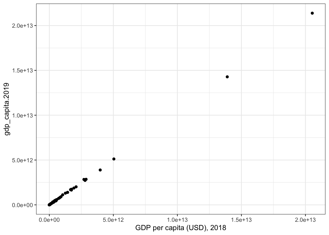
Now that we have this in wide format, we can make that scatterplot:
ggplot(world_bank, aes(x = gdp_capita.2018, y = gdp_capita.2019))+geom_point()+labs(x ="GDP per capita (USD), 2018", x ="GDP per capita (USD), 2019")+theme_bw()
Figure 10.1: Comparison of GDP per capita in 2018 and 2019. It looks like a pretty strong association!
Now that we have our figure built, we might want to reshape the dataset long again to run some models. This is slightly tricky. We unfortunately, can’t just reshape by year. Instead we have to reshape into the longest format possible again with both a variable and year column. From there we can then reshape wide again to get the kind of country-year dataset we want.
The trick to using pivot_longer with multiple desired name variables (e.g. variable and year) is to use that separator information in the argument names_sep above to tell pivot_wider where to split each column name to produce two different columns in the long format. There is a slight issue here however, because the “.” is a special character and it won’t be handled correctly unless I “double-escape” it by using two backslashes in front. The full code to get the longest format possible is:
# A tibble: 434 × 6
   country_name   country_code year     gdp_capita life_exp carbon_emissions
   <chr>          <chr>        <chr>         <dbl>    <dbl>            <dbl>
 1 Afghanistan    AFG          2018   18053222735.     63.1            0.299
 2 Afghanistan    AFG          2019   18799444415.     63.6            0.298
 3 Albania        ALB          2018   15156424015.     79.2            1.85
 4 Albania        ALB          2019   15401826127.     79.3            1.75
 5 Algeria        DZA          2018  174910684782.     76.1            3.92
 6 Algeria        DZA          2019  171760275467.     76.5            3.99
 7 American Samoa ASM          2018     639000000      NA             NA
 8 American Samoa ASM          2019     647000000      NA             NA
 9 Andorra        AND          2018    3218418632.     NA              6.59
10 Andorra        AND          2019    3155150256.     NA              6.29
# ℹ 424 more rows
Reshaping data can be a bit tricky sometimes, but if you can get the dataset into its longest format possible, you can always get it in the ultimate shape that you want.
Aggregating Data
Lets go back to the American Community Survey data that we have been working on for the last few chapters to better understand how to aggregate data. Let me just load and clean up taht data here for our use.
# A tibble: 100,106 × 5
   state   sex      age health_ins  degree
   <fct>   <fct>  <int> <fct>       <fct>
 1 Alabama Male      51 Covered     HS
 2 Alabama Female    19 Covered     HS
 3 Alabama Male      50 Covered     HS
 4 Alabama Female    56 Covered     HS
 5 Alabama Female    93 Covered     HS
 6 Alabama Male      62 Covered     HS
 7 Alabama Male      18 Covered     HS
 8 Alabama Male      20 Covered     HS
 9 Alabama Male      53 Covered     LHS
10 Alabama Male      56 Not covered HS
# ℹ 100,096 more rows
We have a few interesting variables on individuals from the American Community Survey data. Importantly, we have a variable that identifies each individual’s state of residence. Instead of individual data, we might want to get an aggregate dataset of states that includes summary information on the variables. For example, lets say we want a dataset to analyze differences in health insurance coverage across states. We could estimate a state level estimate of the proportion of the population covered by health insurance.
To do this in R we are going to use two commands. The first command is group_by command that tells us what variable or variables we want to aggregate across. In this case, the variable is state.
acs |>group_by(state)
# A tibble: 100,106 × 5
# Groups:   state [50]
   state   sex      age health_ins  degree
   <fct>   <fct>  <int> <fct>       <fct>
 1 Alabama Male      51 Covered     HS
 2 Alabama Female    19 Covered     HS
 3 Alabama Male      50 Covered     HS
 4 Alabama Female    56 Covered     HS
 5 Alabama Female    93 Covered     HS
 6 Alabama Male      62 Covered     HS
 7 Alabama Male      18 Covered     HS
 8 Alabama Male      20 Covered     HS
 9 Alabama Male      53 Covered     LHS
10 Alabama Male      56 Not covered HS
# ℹ 100,096 more rows
So far, the output seems like the same dataset that we started with. However, hyou will notice an additional header saying Groups: state [50]. This tells us that we now have a grouped tibble object. This object has information about our grouping and we can now apply the summarize command to summarize characteristics across groups. Typically we would apply both group_by and summarize in a pipe.
I now have a dataset with 50 observations, one for each state and one variable p_health_cover which gives me an estimate of health insurance coverage in each state.
You can arbitrarily summarize as many things as you want in the summary command. The basic syntax is a name = value pair where name is the name of the summary variable you are creating and value is a function applied to one of the statistics to create a summary measure. In this case, I am taking the mean of a TRUE/FALSE variable which gives me a proportion. I could add other summary statistics to this aggregate dataset as well, separating them by commas.
You can also group by more than one variable at a time. For example, I might be interested in looking at health coverage for men and women separately by state to identify different gender gaps in coverage. By adding sex to the group_by command, I can get a dataset aggregated along two dimensions.
# A tibble: 100 × 3
# Groups:   state [50]
   state      sex    p_health_cover
   <fct>      <fct>           <dbl>
 1 Alabama    Male            0.898
 2 Alabama    Female          0.934
 3 Alaska     Male            0.920
 4 Alaska     Female          0.914
 5 Arizona    Male            0.870
 6 Arizona    Female          0.914
 7 Arkansas   Male            0.866
 8 Arkansas   Female          0.928
 9 California Male            0.928
10 California Female          0.952
# ℹ 90 more rows
This is interesting, but what if we want to calculate the difference in proportion coverage between men and women? We can’t do that with this dataset because men and women are showing up on different lines. However, you may recognize that what we have here is a particularly kind of long dataset. We have a particular value (p_health_cover) organized by state and gender. So, we can apply what we have learned above about reshaping to reshape this into a wide dataset where men’s and women’s values are on the same row.
We can now see that the biggest difference in coverage is in Oklahoma, and that generally men are less likely to be covered than women. Likely this difference is at least partly owing to the fact that women are older than men on average due to longer life expectancy and are thus more likely to be covered under Medicare. However, we could slice age into intervals here and add that to the group_by command to check that more formally. I will leave that as an exercise for those so inclined.