Appendix A — Getting Familiar with RStudio

In this book, we use the statistical programming language R within the RStudio Integrated Development Environment (IDE). An IDE is an application that makes it easier to work with code by giving you access to a variety of different additional features. RStudio will do that for us.

R itself is an open source statistical programming language that is built from an earlier statistical programming language called S (and later S-plus). S was designed to mimic many of the features of the C++ programming language, while offering a variety of built-in functions to make statistical analysis straightforward. With the creation of the tidyverse, R has now become one of the major players in data science and statistical analysis. Unlike S/S-plus which was owned by Bell labs, R is not owned by anyone in particular and is instead developed by an a community of open source developers and statisticians.

RStudio is developed by Posit. Posit used to just be named RStudio, which gives you a sense of how much they value this product. The company was also founded by Hadley Wickham, who created ggplot and the tidyverse. While you can big bucks for “enterprise” versions, the basic RStudio Desktop version is completely free to use.

To install R and RStudio, simply go here and follow the instructions. Both R and RStudio are available on all major platforms. You can also run RStudio over a web browser using posit.cloud, but I would prefer you first learn how to use it on a local machine.

The RStudio Interface

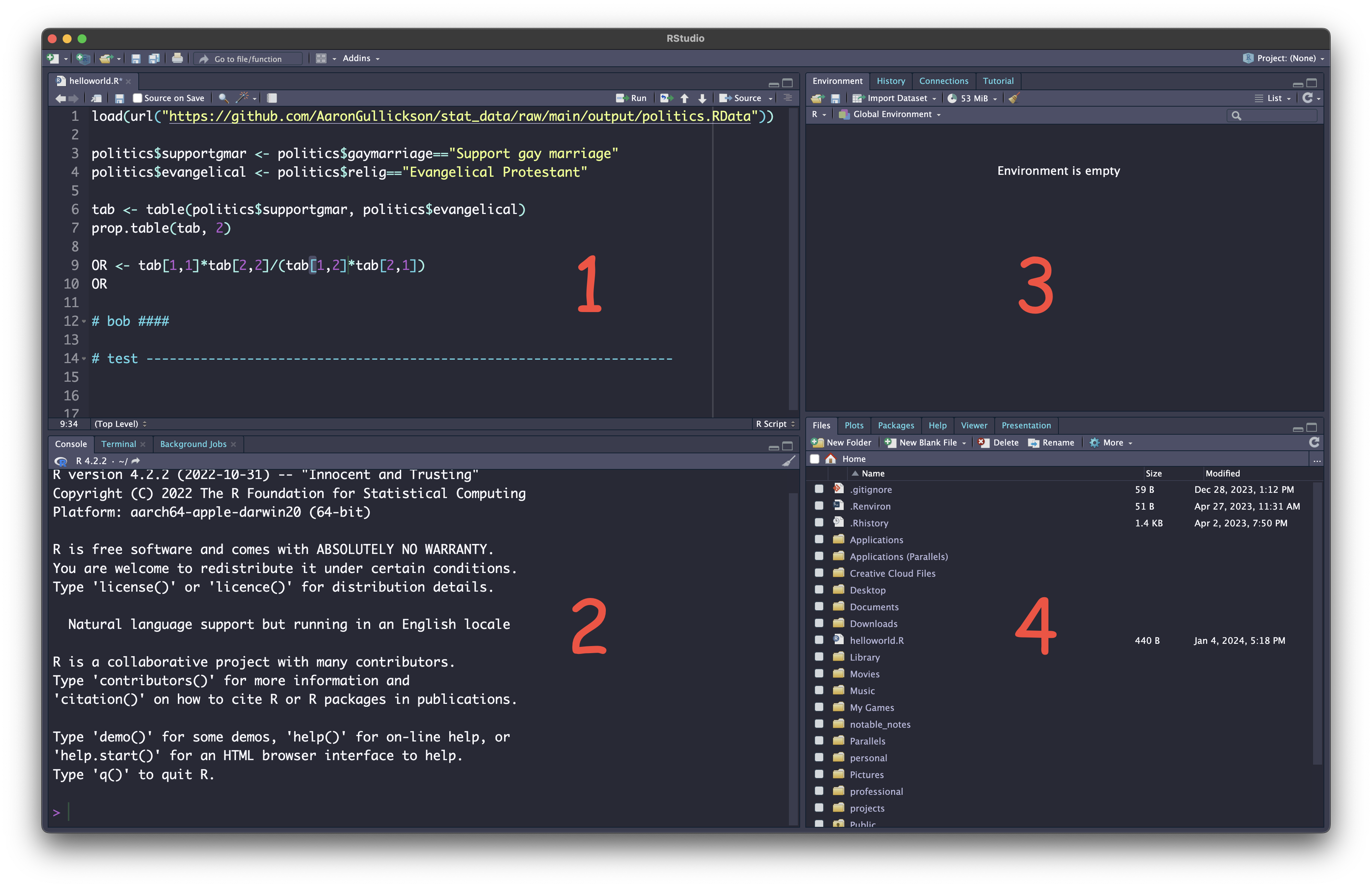
Figure A.1 shows a typical RStudio screen. When you have a document opened, you will be presented with four different panels, which are numbered in Figure A.1 above. Each of these panels, also has multiple tabs. You can actually customize where things show up if you don’t like the default layout. However, I would recommend using the default layout while learning in this course.

Let’s discuss what you will find in each of the panels, by number:

This is the editor panel. You can open up files here like scripts and quarto files. RStudio will let you edit any plain-text document in this editor. When you first open RStudio, you may not see this editor because you do not have an open document. Just go to File > New File > R Script to see this panel. You can also have multiple documents open at the same time in different tabs. So like everything else in your life, you can have too many tabs open in RStudio too!
R itself lives in this panel. This is what R looks like. It is just a command line interface. so you should be presented with a prompt (>) and a blinking cursor waiting for your fine instructions. You can type your command directly into the console here. However, we more commonly run our commands from a script in the upper left panel as described in Chapter 3. You should also see another tab here that says “Terminal.” This tab can be used for interacting directly with your operating system command line interface. Generally, you won’t need to do this unless you need to run git from the command line for some reason.
The upper right panel has several tabs. The default tab, “Environment”, shows all of the objects that are currently loaded into memory. The other important tab that lives in the upper right panel is the “Git” tab which will allow us to interact with git, as described in Chapter 2. You don’t see that in Figure A.1 because I am not in a git repository.
The lower right panel has several useful tabs. The default tab allows you to navigate around your file system. The “Help” tab is also very useful as you can search through R commands here and read help files. When you make figures in R, they will be displayed in the “Plots” tab.

Where is Your Working Directory?

R always operates in a specific working directory. If you ask it to a load a file by name, it will expect that file to be in its working directory. If you save a plot as an image file, it will be default save to the working directory. You should always know what your working directory is and how to change it.

So how do you know what working directory you are in? You can type the following into the R console to identify your working directory:

getwd()

[1] "/Users/aarong/teaching/practical_analysis"

It is reporting the full path to my working directory from the base of my computer. So I am in “practical_analysis” directory which is a subdirectory of the “teaching” directory which is a subdirectory of the “home” directory of user “aarong” (thats me!).

However, you don’t even need to run this command. If you look at the top of your console tab, you will see that it shows your current working directory right there, as shown in Figure A.2.

Figure A.2: Information at the top of your R console will show you the current working directory. The `~` is short for your user’s home directory.

Save Your Work!

RStudio does not autosave documents, so you need to be sure to save your work periodically as you are working on it. You can do this with File > Save from the menu, with the floppy disk icon at the top, or with Control+S (or Command+S on Mac).

You can tell when a document has unsaved changes because its name in the tab at the top of the editor panel will have an “*” next to it, and may change color in some themes.

If you do try to quit without having saved changes, a reminder will pop up to save your work, but don’t rely upon this. Make it a habit to save frequently.

Changing Preferences

RStudio has a huge variety of customizability. To see all the things you can customize, go to Tools > Global Options from the menu. Under the Appearances tab, you can customize your color theme and other appearance issues. There are a couple of other settings that I would highly recommend you change from their defaults:

On the General tab you will see an option to “Save workspace .RData on exit.” I strongly recommend that you set this to “Never.” I would also uncheck “Restore .Rdata into workspace on startup.” Historically, this was a way to save all of the objects that you were working on to a hidden file called .RData and then have them available the next time you start R. This is a bad way to ensure that you can reproduce your work however, and can lead to long start up times and a giant hidden file on your system if you have a bunch of enormous objects in there.
On the Code > Display tab, I recommend you check the “Show Margin” option and set your margin at 80 characters. This will create a vertical line that lets you know when you are at 80 characters on a line. We try to keep lines 80 characters of less and this will enforce that practice.
In the R Markdown tab, I recommend you change “Show Output Preview in:” to “Viewer Pane. That will prevent an annoying pop-up window every time you render a Quarto document.