a <- 33 Learning R Basics
In this chapter, I will cover the basics of “base” R. In the next chapter, we will build on this foundation to learn additional features available from a set of packages known as the “tidyverse.” If you have not done so already, it may be useful to review Appendix A to understand the basic structure of RStudio and how to interact with R.
Creating Objects
R is an object-oriented language. In simple terms, that means we can create a variety of different “objects” and then apply commands or methods to these objects. To create an object, we use the assign syntax of <- to assign something to a named object. For example:
I have now assigned the numeric value of 3 to an object called a. Note that I could have called this object anything I wanted so long as it was one word (e.g. bob, value). This object will now show up in the environment tab of RStudio as an object loaded into memory.
Note that when you type this into the console, the console will just move on to the next prompt without further output. That is because you assigned the value to an object. If you want to see what is in the object, you can just provide the object name itself and hit return to print its contents to the screen.
a[1] 3I can then use this variable in other ways, such as:
a+2[1] 5R is smart enough to realize that I want to add 2 to the value in a, and reports that the result is 5.
If you are looking for the <- key on your keyboard, you are searching in vain. This symbol is created by combining the less than (<) and dash (-) signs. You can also use a single equals sign = to indicate assignment. The = is a more common assignment operator in many computer languages, but using <- is the norm in R.
Objects can come in many different forms. By far the most common object you will use throughout this book and in your daily practice is some form of a data.frame which has the typical format we expect of a dataset - observations on the rows and variables on the columns. However, the data.frame object is a complex object composed of several other different object types. Its useful to build from the ground up the different kinds of standard object types that you will encounter in R.
Atomic Types
The atomic types are the building blocks for other more complex objects. The three most important atomic types for our purposes are:
numeric-
records a numeric value.
character-
records a set of characters. This is often called a string or character string in computer science parlance.
logical-
records either a TRUE or FALSE value. In computer science parlance, this is called a boolean.
Lets try creating one of each of these types in R.
a <- 3.14        # numeric type
b <- "bob said"  # character string type
c <- TRUE        # logical type, must be TRUE or FALSE
Note that to create a character string, you must surround it in either single or double quotation marks.
In some cases, you can force, or recast, one type into another with commands that start with as.. For example, lets say I want to turn object a into a character string.
as.character(a)[1] "3.14"It still looks like a number but the quotes give us a hint that it is actually a character string. As a result you cannot perform math on it as we did above:
as.character(a)+2Error in as.character(a) + 2: non-numeric argument to binary operatorWe can also force logicals into numeric values where TRUE=1 and FALSE=0. Alternatively, if we have a 1 or 0 numeric value, we can recast it as a logical.
as.numeric(c)[1] 1as.logical(0)[1] FALSEHowever, you can’t recast a character string as anything else:
as.numeric(b)[1] NAThe result here is an NA value which is a special value tracked in R and generally used for missing values.
Vectors
You can combine a bunch of values of the same atomic type together into a single vector. A vector is what we use to record all of the values for a single variable.
To manually construct a vector, you can use the concatenation function c(). Inside the parenthesis we put all the values we want, separated by commas. Lets do that to create several variables for a fictitious dataset.
name <- c("Bob", "Juan", "Maria", "Jane", "Howie")
age <- c(15, 25, 19, 12, 21)
ate_breakfast <- c(TRUE, FALSE, TRUE, TRUE, FALSE)
One thing to note is that the atomic type of each value must be the same. if you feed in different atomic types to the same vector, R will recast them to a shared common type. For example:
x <- c(TRUE, "bob", 3)
x
[1] "TRUE" "bob" "3" All of the values became character strings, because that was the only type to which they could all be recast.
Many functions that we use in data analysis expect a vector of values as input. A useful example is the mean which will calculate the mean of a vector of values:
mean(age)[1] 18.4mean(ate_breakfast)[1] 0.6A mean for the age variable makes sense, but how did R calculate the mean of the ate_breakfast vector? R attempted to recast the vector into a numeric type, which led to a vector of zeroes and ones. The mean here is equivalent to the proportion of true values. So 60% of respondents ate breakfast.
Vectors are one-dimensional objects with a length (i.e. the number of values). The length function will tell you how many values are in a given vector.
length(age)[1] 5You can also include NA values in a vector to indicate missing values:
height <- c(67, NA, 64, 66, 72)Notice that I do not surround the NA value with quotation marks, which would convert the entire vector into a character string type. The raw NA value is a special value that R knows how to store in memory.
If you want to retrieve a specific value from your vector, you can do it by the index. You do this by including square brackets after the name of the vector and inside of the square brackets, you include the index number of the value. The index number starts at 1 in R and goes up. So, if I wanted to identify the name of the third respondent:
name[3][1] "Maria"You can also use a vector of numbers here to identify multiple indices at once:
name[c(1,4)][1] "Bob" "Jane"One useful shortcut in R is the a:b syntax which will give you each integer between a and b. For example, if I wanted the third through fifth respondent:
name[3:5][1] "Maria" "Jane" "Howie"Matrices
A matrix is just an extension of a vector into two dimensions. We can use the matrix command to turn a vector into a matrix, by specifying the number of rows and columns.
x <- matrix(c(4,5,3,9,7,8), 3, 2)
x
[,1] [,2]
[1,] 4 9
[2,] 5 7
[3,] 3 8I can also create a matrix by binding together vectors into different rows (rbind) or columns (cbind).
a <- c(4,5,3)
b <- c(9,7,8)
cbind(a,b)
a b
[1,] 4 9
[2,] 5 7
[3,] 3 8rbind(a,b) [,1] [,2] [,3]
a 4 5 3
b 9 7 8A matrix may seem like a natural way to represent a full dataset. However, there is an immediate problem if I attempt to do this by using cbind on the variables I created earlier.
cbind(name, age, ate_breakfast) name age ate_breakfast
[1,] "Bob" "15" "TRUE"
[2,] "Juan" "25" "FALSE"
[3,] "Maria" "19" "TRUE"
[4,] "Jane" "12" "TRUE"
[5,] "Howie" "21" "FALSE" Like a vector, all the values in a matrix must be of the same atomic type. In most cases, if there is any character vector in the binding, everything will be recast into character stings, which is not every useful. We will see a better way to create a dataset with the data.frame object below.
You can extract values from a matrix by indexing just like a vector. However, because a matrix is two dimensional, you need to include a comma inside the square brackets. Values before the comma indicate row indices and values after the comma indicate column indices. If you leave the values in one dimension blank you will get all of the rows/columns.
#value in 2nd row, 1st column
x[2, 1]
[1] 5#2nd row
x[2,][1] 5 7#1st column
x[,1][1] 4 5 3#1st and 2nd row
x[1:2,] [,1] [,2]
[1,] 4 9
[2,] 5 7Factors
You can easily represent quantitative variables with a numeric type vector, but how do you represent categorical variables? Lets say for example that I wanted to include highest degree received for my respondents from above. I could create this as a character variable:
high_degree <- c("Less than HS", "College", "HS Diploma", "HS Diploma",
                 "College")
summary(high_degree)
Length Class Mode
5 character character The values of the character string indicate categories of my categorical variable. However, R will not be able to do much with this variable as you can see from the summary command. To represent categorical variables, we instead want to use a factor.
A factor in R is the standard type for coding categorical variables. Each value is actually recorded as a numeric value but the factor object also contains a set of labels that link the numeric values to category names. Most functions in R will then know how to handle factors intelligently.
To create a factor object, I can just apply the factor function to my vector:
high_degree_fctr <- factor(high_degree)
levels(high_degree_fctr) # return levels of factor
[1] "College" "HS Diploma" "Less than HS"summary(high_degree_fctr) College HS Diploma Less than HS
2 2 1 Now the summary command gives me a table of frequencies for each category.
The only problem with my factor is that the underlying categorical variable is an ordinal variable and the categories are backwards with “College” first and “Less than HS” last. This is because R sorts alphabetically by default. In order to ensure a specific order to the categories in the factor, I will need to specify the levels argument in the factor function and explicitly write out the order I want:
high_degree_fctr <- factor(high_degree,
                           levels=c("Less than HS", "HS Diploma", "College"))
levels(high_degree_fctr)
[1] "Less than HS" "HS Diploma" "College" summary(high_degree_fctr)Less than HS HS Diploma College
1 2 2 The factor levels are now appearing in my desired order.
Watch for Mispelled Factor Levels!
When specifying levels manually, you will need to be careful to spell the categories exactly as they appear in the names. When converting character strings to factors, if there is no corresponding factor level for a character string, it receives an NA value. If you see that a large number of your observations went into a missing value code and a category is missing from your final factor, you likely misspelled or forgot a level.
For example, lets intentionally misspell “HS Diploma” by not capitalizing the second word:
high_degree_miss <- factor(high_degree,
                           levels=c("Less than HS", "HS diploma", "College"))
summary(high_degree_miss)
Less than HS HS diploma College NA's
1 0 2 2 You can see that we now have no observations in the “HS diploma” category and two missing values (which are actually HS diploma holders).
Lists
Lists are one of the most flexible types of standard objects. Lists are just collections of other objects and the objects can be of different types and dimensions. You can even put lists into lists and end up with lists of lists (or go crazy and make lists of lists of lists).
Lets put the five variables we have created so far into a list:
my_list <- list(name, age, ate_breakfast, high_degree_fctr, height)
my_list
[[1]]
[1] "Bob" "Juan" "Maria" "Jane" "Howie"
[[2]]
[1] 15 25 19 12 21
[[3]]
[1] TRUE FALSE TRUE TRUE FALSE
[[4]]
[1] Less than HS College HS Diploma HS Diploma College
Levels: Less than HS HS Diploma College
[[5]]
[1] 67 NA 64 66 72In this case, each item in the list is a vector of the same length, but that is not required.
You will notice a lot of brackets in the list output above. To access an object at a specific index of the list, I need to use double square brackets. Lets say I wanted to access the third object (ate_breakfast):
my_list[[3]][1] TRUE FALSE TRUE TRUE FALSEIf I want to access a specific element of that vector, I can follow up that double bracket indexing with single indexing:
my_list[[3]][4][1] TRUEMy fourth respondent did eat breakfast. Good to know.
There is another way to access objects within the list but to do this, I need to provide a name for each object in the list. I can do this within the initial list command by using a name = value syntax for each object:
my_list <- list(name = name, age = age, ate_breakfast = ate_breakfast,
                high_degree = high_degree_fctr, height = height)
Now, I can call up any object by its name with the syntax list_name$object_name. Lets do that for age:
my_list$age[1] 15 25 19 12 21mean(my_list$age)[1] 18.4You will notice in RStudio that when you type the “$”, it brings up a list of all the names you might want. You can select the one you want and tab to complete. Thanks, RStudio!
Data Frames
The list was not an ideal way to represent my dataset because it didn’t represent data in the two-dimensional observations-on-the-rows and variables-on-the-columns way we expect most datasets to be organized. This is where the data.frame object comes in. This is the object that we work most directly with for data analysis. In practice, when we move to the tidyverse approach in the next chapter, we will use an extension of the data.frame called a tibble but we will start in this chapter with the basic data.frame.
The data.frame object is basically a special form of a list in which each object in the list is required to be a vector of the same length, but not necessarily of the same type. The results are displayed like a matrix and the same kinds of options for indexing that are available for matrices can be used on data.frames.
Lets put our variables into a data.frame:
my_data <- data.frame(name, age, ate_breakfast, high_degree = high_degree_fctr,
                      height)
my_data
name age ate_breakfast high_degree height
1 Bob 15 TRUE Less than HS 67
2 Juan 25 FALSE College NA
3 Maria 19 TRUE HS Diploma 64
4 Jane 12 TRUE HS Diploma 66
5 Howie 21 FALSE College 72Now that looks like a dataset! The display shows us the expected “spreadsheet” look with observations on the rows and variables on the columns. The type of each variable has been preserved. Note that by default, it just used the name of the object as the column name. However, I specifically changed this behavior for high_degree_fctr with the same name=object syntax I used for lists.
We can run a summary on the whole dataset now and get some nice output.
summary(my_data) name age ate_breakfast high_degree
Length:5 Min. :12.0 Mode :logical Less than HS:1
Class :character 1st Qu.:15.0 FALSE:2 HS Diploma :2
Mode :character Median :19.0 TRUE :3 College :2
Mean :18.4
3rd Qu.:21.0
Max. :25.0
height
Min. :64.00
1st Qu.:65.50
Median :66.50
Mean :67.25
3rd Qu.:68.25
Max. :72.00
NA's :1 I can also access any specific variable with the same $ syntax I used for lists:
my_data$age[1] 15 25 19 12 21mean(my_data$age)[1] 18.4I can also define new variables in my dataset with the same $ syntax and the assignment operator:
my_data$age_squared <- my_data$age^2I can also use the same indexing as for matrices to retrieve particular values. Columns can also be referenced by their name rather than index.
my_data[c(1, 3),] # first and third observations name age ate_breakfast high_degree height age_squared
1 Bob 15 TRUE Less than HS 67 225
3 Maria 19 TRUE HS Diploma 64 361my_data[c(1, 4), "height"] # height of first and fourth observations[1] 67 66my_data[,c("age", "height")] # age and height of all observations age height
1 15 67
2 25 NA
3 19 64
4 12 66
5 21 72Boolean Statements
One of the most important features in all computer programming languages is the ability to create statements that will evaluate to a “boolean” value of TRUE or FALSE (a “logical” value in R parlance). These kinds of statements are called boolean statements. Table 3.1 shows the basic operators you can use to make boolean statements in R.
| Operator | Meaning |
|---|---|
| == | equal to |
| != | not equal to |
| < | less than |
| > | greater than |
| >= | less than or equal |
| <= | greater than or equal |
Note that the “equal to” syntax is two equal signs together. This syntax is necessary because a single equal sign can be used for assignment of values to objects.
As a simple example, lets say that I wanted to identify all respondents from my data above that were 18 years of age or older:
my_data$age >= 18[1] FALSE TRUE TRUE FALSE TRUEI can see that the second, third, and fifth respondents were 18 years or older.
You can use factor variables in boolean statements of equality as well, but you need to use character strings matching the names of the levels. Lets say I want to identify all respondents with a college degree:
my_data$high_degree == "College"[1] FALSE TRUE FALSE FALSE TRUEA very important feature of boolean statements is the ability to string together multiple boolean statements with an & (AND) or | (OR) to make a compound statement. Lets say I wanted to identify all respondents who had either a high school diploma or a college degree:
my_data$high_degree == "College" | my_data$high_degree == "HS Diploma"[1] FALSE TRUE TRUE TRUE TRUELets say I want to find all respondents who are between the ages of 20 (inclusive) and 25 (exclusive):
my_data$age >= 20 & my_data$age < 25[1] FALSE FALSE FALSE FALSE TRUEYou can (and generally should) use parenthesis to ensure that your compound boolean statements are interpreted in the correct order.
(my_data$age >= 20 & my_data$age < 25) &
  (my_data$high_degree == "College" | my_data$high_degree == "HS Diploma")
[1] FALSE FALSE FALSE FALSE TRUEAnother useful option is the ability to put a ! sign in front of a logical variable to indicate “not”. Lets say I wanted to find all respondents who had not eaten breakfast:
!my_data$ate_breakfast[1] FALSE TRUE FALSE FALSE TRUEUsing Functions
We have already seen a couple of functions in the previous sections. Functions are predefined bits of code that take some kind of input and give you output. Base R has many, many functions for doing statistical analysis and data wrangling. Additional packages, which I discuss below, add more functions.
The syntax of a function is:
function_name(argument1, argument2, argument3, ...)The function is identified by the opening and closing parenthesis after its name. Within those parenthesis you may feed in arguments that the function will process. Not all functions need arguments, so you may run into cases where you just have an empty parenthesis. Some functions can take many arguments and so the arguments should be separated by commas.
Lets look at one of the functions we have already seen - the mean function. This function will calculate the mean of a vector of numbers.
mean(my_data$age)[1] 18.4In this case, the function only needed a single argument which was the actual vector of data for which I want the mean. However, in some cases, you may need additional arguments. Lets try the mean function for the height data.
mean(my_data$height)[1] NAIt reports an NA because some of the values in this vector are NA. You might think a reasonable behavior would be to drop the NA values and just calculate the mean of the non-missing values. The mean function can in fact do this but not as its default behavior. It wants to make sure you are aware of the missing value in this variable.
Every function has a help file that will give you information about the function and the arguments that it can take. To view the help file just give the name of the function with no parenthesis and preceded by the question mark. So to pull up the help file for the mean, you can type:
?mean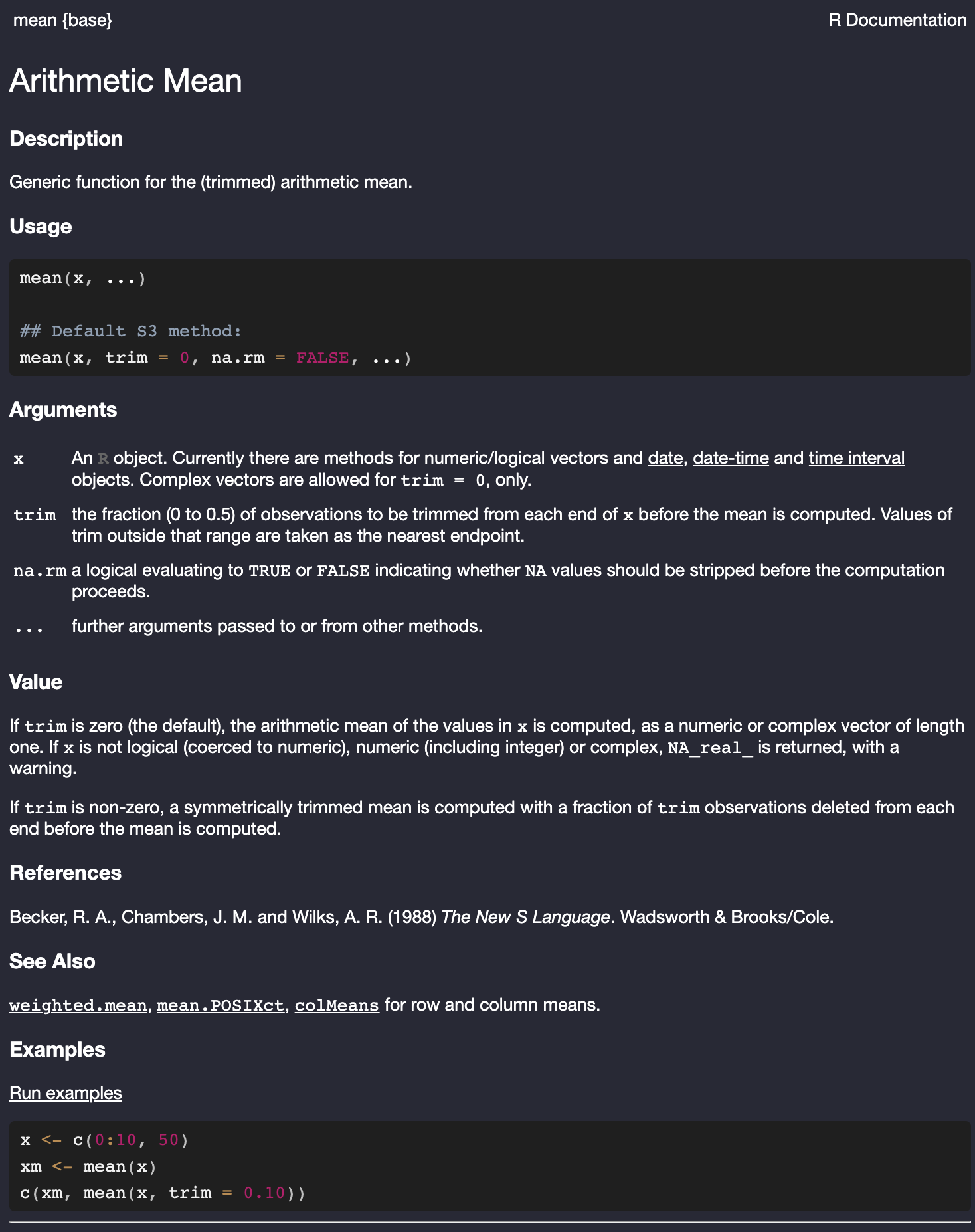
mean function in R.
Figure 3.1 shows the help file for the mean function. Most importantly, we want to look at the arguments section that describes the arguments we can feed into the mean function. You can see here that the first expected argument is a numeric or logical vector (described as x). The third argument is named na.rm and takes a logical value. If TRUE it will strip out NA values before computation. That is the behavior we want. However, if you look to the Usage section of the help file, you can see that this argument is set to FALSE by default. So, we need to change that value to TRUE.
To do that, we need to understand how R matches arguments. If I don’t name my arguments, which I have not so far, R will process the arguments in the expected order shown in the Usage section of the help file. I haven’t needed to do that so far, because the mean function expects my vector to be the first argument. However, I now want to change the value of the third argument without messing with the second trim argument. I can do this by feeding in the argument with a name. The syntax for this is arg_name=arg_value. In this case, I need to use na.rm=TRUE. So, to get the mean of height with missing values dropped, I need:
mean(my_data$height, na.rm=TRUE)[1] 67.25There we go! For the non-missing values, the mean height was 67.25 (inches, presumably).
We will cover many functions throughout the course. The help file can remind you how to use functions if you forget. The Examples section of the help file is particularly useful as it will provide executable examples of how to use a function.
Keep in mind that the output of a function will be some kind of object. You can save that output just like any other object. This will be particularly useful when we get to model building as we can save the output of our model estimation and run a variety of additional functions on it.
Making Scripts
One of the primary advantages of using a statistical programming language like R, Stata, or python is the ability to conduct your analysis in a script. A script is a text file of commands that can be run to do a thing, whether that be some data cleaning, running models, or making a figure. It is good practice to always do your work using scripts. The advantage of scripting is that you will have an easily reproducible record of exactly what you did.
You should think of a script as an executable bit of code that does something. It should have a beginning and an end. Running through the commands in the script will walk the user through the thing that the script does. You should most definitely not think of your script as a set of notes and random bits of code that you want to remember. While, you may in some cases use scripts that way for learning purposes, for actual research a script should just work, with only the code needed to make it work.
A First Script
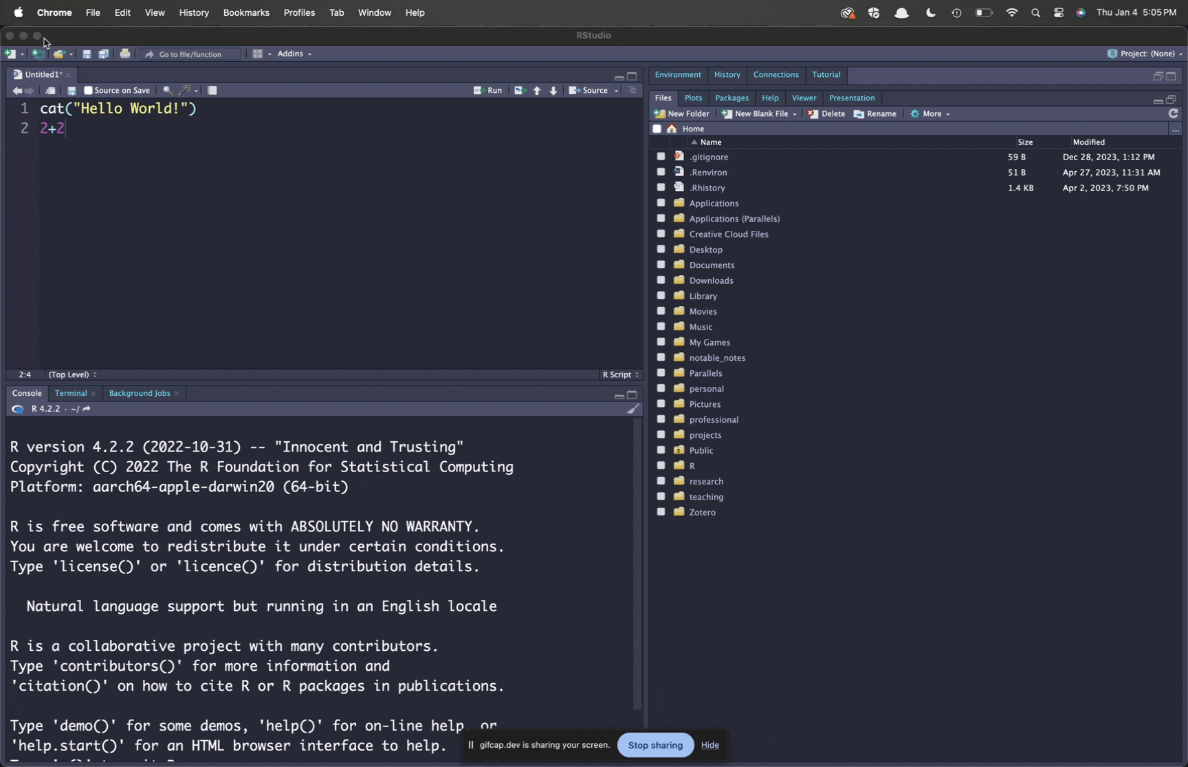
Lets put together a simple “Hello World! script. To create and open a new script in RStudio, go to File > New File > R Script as shown in Figure 3.2.
Lets start by writing a simple “Hello World” script. Type the following command into your script:
cat("Hello World!")
2+2
We now have code from our script in the upper left pane; and the R console waiting for that delicious code in the lower right panel. How can we get it there? You can run the code in this script a couple of different ways:
- You could just copy and paste both lines of code to the console manually. This is quick and dirty but is typically not the most efficient way to run code from your script.
- You could run your entire script by clicking the “Source” button in the upper right corner of the script panel. Note that with this button, you won’t get the output, unless you use the drop-down arrow to choose “Source with Echo.”
- You could run a single line of your script where the cursor is located. You can do this by either hitting the “Run” button or by clicking Ctrl+Enter on Windows/OSX or Command+Enter on OSX. When you do execute the code this way, your cursor will automatically move to the next line of code, so you can execute your way through the code simply by clicking Ctrl+Enter repeatedly. Generally, this is the best approach to running your code line by line.
- If you have saved the script to a file, you can also type in the
sourcecommand in the console to source the script.
Figure 3.3 shows different ways to execute the code in your script.
A Slightly More Complicated Script
Now lets try a slightly more useful script. In this script, I am going to use the politics dataset to do the following:
- re-code the gay marriage support variable into support for gay marriage vs. all else, and the religion variable as evangelical vs. all else
- Create a two-way table (crosstab) of these two new variables.
- Calculate the odds ratio between the two new variables.
I don’t expect you to know how all of this code works yet. I just want to show you an example of a script that actually does something interesting.
load(url("https://github.com/AaronGullickson/stat_data/raw/main/output/politics.RData"))

politics$supportgmar <- politics$gaymarriage=="Support gay marriage"
politics$evangelical <- politics$relig=="Evangelical Protestant"

tab <- table(politics$supportgmar, politics$evangelical)
prop.table(tab, 2)
            FALSE      TRUE
  FALSE 0.3355322 0.7184035
  TRUE  0.6644678 0.2815965
OR <- tab[1, 1]*tab[2, 2]/(tab[1, 2]*tab[2, 1])
OR[1] 0.1979334If I source this script, I will get:
> load(url("https://github.com/AaronGullickson/stat_data/raw/main/output/politics.RData"))
> politics$supportgmar <- politics$gaymarriage=="Support gay marriage"
> politics$evangelical <- politics$relig=="Evangelical Protestant"
> tab <- table(politics$supportgmar, politics$evangelical)
> prop.table(tab, 2)
FALSE TRUE
FALSE 0.3355322 0.7184035
TRUE 0.6644678 0.2815965
> OR <- tab[1, 1]*tab[2, 2]/(tab[1, 2]*tab[2, 1])
> OR
[1] 0.1979334About 66% of non-evangelicals support gay marriage while only 28% of evangelicals support it. That works out to an odds ratio of 0.198, meaning that the odds of gay marriage support were about a fifth as high for evangelicals as for non-evangelicals.
Not Everything Goes Into Your Script
You don’t need to put every command into your script. The script should provide a narrative of your analysis (the part that you want to be easily reproducible), not a log of every single command you ran. Sometimes you may try out some exploratory commands or may just need to get some basic information about a variable. For example, in the script above, I first had to remember what the names were for the categories of the gaymarriage variable. To figure this out, I typed:
levels(politics$gaymarriage)From there I could see that the category I wanted was called “Support gay marriage” and I could use that in my script. However, there was no need to put this command into my script. This kind of interactive coding belongs in the console not in the script.
Commenting for Clarity
There is one big thing missing from the scripts listed above: comments! Comments are crucial for good script writing. Comments are lines in your script that will not be processed by R. You can create single line comments by using the pound sign (#). Anything after the pound sign will be ignored by R until a new line. You should use these comments to explain what the code is doing. You can also use them to help visually separate the script into sections for easier readability. Comments help you remember what you were doing when you come back to a project you haven’t worked on for weeks or months. They are also useful for other people who might end up reading your code (co-authors, advisers, etc).
Here is the script from above, but now with some helpful commenting:
#################################################################
# Aaron Gullickson
# Program to analyze the differences in support for gay marriage
# between evangelical christians and all those of other religious
# affiliations
#################################################################
# Data Organization --------------------------------------------------------
#load the politics dataset directly from its GitHub repository
load(url("https://github.com/AaronGullickson/stat_data/raw/main/output/politics.RData"))
#dichotomize both the support for gay marriage and the religious variable
politics$supportgmar <- politics$gaymarriage=="Support gay marriage"
politics$evangelical <- politics$relig=="Evangelical Protestant"
# Analysis -----------------------------------------------------------------
#create a crosstab
tab <- table(politics$supportgmar, politics$evangelical)
#Distribution of support conditional on religion
prop.table(tab, 2)
#Calculate the odds ratio of support
OR <- tab[1, 1]*tab[2, 2]/(tab[1, 2]*tab[2, 1])
OREven if you don’t understand what the code here is doing yet, you can at least get a sense of what it is supposed to be doing. Notice that I use multiple pound signs to draw attention to the header and larger sections. For a script this small, the division between Data Organization and Analysis is probably overkill, but for larger scripts, this sectioning can be useful in helping to easily distinguish different components of the analysis.
One nice feature of RStudio is that if you end your comments with at least four pound signs or dashes at the end, then the outline of your script will show these sections and you can navigate to them. You can also collapse and expand them as needed. You can also go to Code > Insert Section to add sectioning comments in this style.
Don’t Overcomment
While commenting is necessary for good script writing, more commenting is not always better. The key issue is that you need to think of commenting as documentation of your code. If you change the code, you also need to change the documentation. If you change the code, but not the documentation, then you will actually make your code more confusing to other readers. The key takeway is that you should only write documentation that you will actively maintain.
The most common error that novices make is to use comments to describe the results of their code. This is bad practice, because as you make changes to your data and methods, these results are likely to change and if you don’t update your comments, there will be a lack of alignment between your real results and your documentation of the results. Later in the term, we will learn a better way to separate out the reporting of results in a “lab notebook” fashion, from comments in scripts.
Adding Packages
R is an open-source program and anyone can write their own package or library that contains a set of custom functions. You can then install and load these packages to gain access to these additional functions. Thousands of packages exist to extend the basic functionality of R. We already saw one of these in Chapter 2 with the usethis package. The “tidyverse” that we will learn in Chapter 4 is based on a set of packages. Learning how to install and load packages is important for getting the most out of R.
Packages that have been vetted are available on the Comprehensive R Archive Network (CRAN). You can install these packages with the install.packages command. The syntax is as follows:
install.packages("package_name")You want to replace “package_name” here with the actual package name. In RStudio, you can go to Tools > Install Packages… from the menu to get a searchable graphical tool for installing packages from CRAN.
However you install the package, remember that installing the package is not the same as loading the package. To gain access to all of the functions contained within the package, you need to load the package with the library command, like so:
library(package_name)Note that when installing packages, the package name is in quotes but not when you load the library.
Generally, you should load any packages you need in the script at the top of that script. The first section of your script should always basically be a “load libraries” section. When you realize deep into your script that you need another package, the temptation is to just put a library command there. Resist that temptation! Go back to the top of your script and put the library command at the top to load the new package. The reason we do it this way is that we want anyone reading our script to know what package dependencies the script has so that they can install any required packages.
Don’t Put
install.packages Commands in Your Script
A common novice mistake is for students to include the install.packages command in a script where they want to use the package. You should put a library command to load the package, but you should never put an install.packages command in your script. Every time you run your script, the package will be re-installed which is a waste of time.
You can gain access to the functions of an installed package without loading the entire package. The syntax for using a function from a package without loading the whole package is:
package_name::function_name(...)We already saw an example of this in Chapter 2 with the usethis package. For example, to do a git sitep, I told you to run usethis::git_sitrep(). Alternatively, we could have loaded the usethis package and then run git_sitrep(). In the case of usethis, you are often running commands from this package interactively and not through scripting, so being able to call functions without loading the package makes sense.
The other common reason for using this syntax is when you have different packages loaded that have functions with identical names. When this kind of conflict occurs, the function for the more recently loaded package will mask the function from the previously loaded package. To gain access to that masked function you will have to reference the function using this syntax.
Following Norms
Programming languages aren’t just the languages themselves but the community of developers and programmers who code with them. Part of this community development is the creation of norms and standard practices that users of that language come to expect even if they are not required by the syntax. R is no different in that respect. You have seen already in this book and will continue to see certain coding practices that are the norm among R coders. You should follow these practices as well in your coding as it will make your code more legible to others.
The norms I use here are developed from the tidyverse style guide. Here are the norms I want you to follow:
- Naming things (e.g. objects, variables, functions, files)
- Names should be all be lower-case and contain no special characters. To separate distinct words within a name, you should use an underscore
_(sometimes called “snake case”). So, for example, if you have a variable measuring the highest grade a respondent attained, you could name thathigh_gradenotHIGHGRADE,HighGrade, orhigh.grade. The use of the underscore for separation does co-exist with an older norm in R to use the.for separation and you will see that in many function names. However, the tidyverse norm is to use the_(which is one way you can often differentiate tidyverse and base R functions). - When naming things, you should strive for a balance between the name being meaningful and concise. Long object and variable names will make your code harder to read.
- Avoid naming things that are already function names (e.g. don’t name your object “mean”).
- Names should be all be lower-case and contain no special characters. To separate distinct words within a name, you should use an underscore
- Spacing
- Leave one space before and after the assignment operator
<-. - Leave one space after commas, either when indexing or separating arguments in functions.
- Leave one space after the # when writing a comment.
- Leave one space before and after the assignment operator
- Whenever possible, limit your lines of code to 80 characters for better legibility. You can include long lines of code on multiple lines, properly indented. Using Ctrl+I in RStudio will properly indent multi-line commands. To ensure you stay within 80 lines, you can set a visible line in RStudio. Go to Tools > Global Options, then Code > Display. You will see a “Show Margins option with 80 characters set as the default.
Let me show you an example of bad coding practice. In this case, I want to load the politics data and use the cut function to create five-year age groups from the original age variable.
#load the data
load(url("https://github.com/AaronGullickson/stat_data/raw/main/output/politics.RData"))

#break age into 5 year groups
politics$FIVE.Year.Age.Groups<-cut(politics$age,breaks=seq(from=15,to=95,by=5),right=FALSE,labels=paste(seq(from=15,to=90,by=5),seq(from=20,to=95,by=5), sep="-"))
This code works, but it sure is hard to read. There is no spacing at all, so everything is very crunched together. The name of the constructed variable is very long and inconsistent in its naming practice. The load command has to be over 80 characters slightly due to the length of the https address for the data, but the line that does the cutting does not need to be so long. Lets clean all that up using proper style.
# load the data
load(url("https://github.com/AaronGullickson/stat_data/raw/main/output/politics.RData"))

# break age into 5 year groups
politics$age_group <- cut(politics$age,
                          breaks=seq(from=15, to=95, by=5),
                          right=FALSE,
                          labels=paste(seq(from=15, to=90, by=5),
                                       seq(from=20, to=95, by=5),
                                       sep="-"))
Even if you aren’t sure what this code does, its still a lot easier to read, isn’t it?