In this chapter, we want to continue working on the challenge introduced in Chapter 12 of calculating Theil’s H - a measure of racial segregation - for every county in the United States. If you haven’t read that chapter, you should probably do so before continuing on here.
The dataset we used for this analysis is based on tract level data of population counts by race extracted from Social Explorer. You can see a snippet below:
In Chapter 12, we developed a handy function for calculating Theil’s H from census tract data for a given county. This saves us a lot of time and code, because that function allows us to reuse the code for calculating Theil’s H for any county we want. For example, if I want the Theil’s H of Alameda County, California:
tracts |>filter(county_name =="Alameda County, California") |>calc_theil_h()
[1] 0.1689115
However, we still have a bit of a problem. If I want to calculate Theil’s H for all 3,222 counties in the dataset, entering them in one by one is going to be extremely laborious. How can I get R to do the hard work here?
Computers are great at iteration. We basically want to tell R to repeat the same procedure over and over again across all counties in my dataset. There are two approaches to iteration in R: loops and mapping.
Looping
Looping is a common procedure in most computer programming languages. In this case, we want a for loop which will iterate across a vector of values and repeat the same code.1 Here is a simple example of a for loop:
The value i is a placeholder that can be referenced within the for loop itself. The first time the for loop is run, it uses the value of 1 and processes the code in the curly brackets. The next time, the for loop is run, it uses the value of 2, and so on until the final value of 10 is reached.
We want to loop across every county. In order to do that, I need a unique identifier for a county. I could use name or ID in this case. Generally, names are not as reliable, but for more intuitive display, I will use names here as I know that no county names are duplicated within states. To get the unique county names, I can use the unique function:
For expository purposes, I am going to take a small sample of these counties to iterate across so that you don’t have to look at output for all 3,222 counties. Once we get the code working for the small sample, we will go back to the full set.
counties_sample <-sample(counties, 10)
First, lets test out a simple for loop where we print out county names:
for(county in counties_sample) {print(county)}
[1] "Alger County, Michigan"
[1] "Kewaunee County, Wisconsin"
[1] "Catahoula Parish, Louisiana"
[1] "Marshall County, Mississippi"
[1] "Jackson County, Missouri"
[1] "Dakota County, Nebraska"
[1] "Jones County, North Carolina"
[1] "Prince Edward County, Virginia"
[1] "Tipton County, Tennessee"
[1] "Orange County, New York"
Note that I used county rather than i as my placeholder value name because its more intuitive. You can use any name you like here. The for loop seems to be working, so lets try to actually calculate Theil’s H within the loop.
for(county in counties_sample) { tracts |>filter(county_name == county) |>calc_theil_h() |>print()}
That seemed to work. However, at this point, I am just spitting out the results to the screen. I would prefer to save these results back to something. I could just save the results back to a vector, but I would rather save them back to a tibble that includes both the county name and Theil’s H. Either way, I do this by initializing a NULL object and then adding to that object within the loop. For a vector, I can do this by simply concatenating the new value onto the old with c:
theil_h <-NULLfor(county in counties_sample) { h <- tracts |>filter(county_name == county) |>calc_theil_h() theil_h <-c(theil_h, h)}theil_h
However, when I only return a vector, I lose information on which value belongs to which county. Instead, I am going to save the results to a tibble and then use the bind_rows command to add this tibble to my existing tibble:
theil_h <-NULLfor(county in counties_sample) {# calculate Theil's H for this county h <- tracts |>filter(county_name == county) |>calc_theil_h()# add this county's values to our dataset of values theil_h <- theil_h |>bind_rows(tibble(county_name = county, theil_h = h))}theil_h
# A tibble: 10 × 2
   county_name                    theil_h
   <chr>                            <dbl>
 1 Alger County, Michigan          0.136
 2 Kewaunee County, Wisconsin      0.0663
 3 Catahoula Parish, Louisiana     0.0982
 4 Marshall County, Mississippi    0.143
 5 Jackson County, Missouri        0.228
 6 Dakota County, Nebraska         0.136
 7 Jones County, North Carolina    0.0213
 8 Prince Edward County, Virginia  0.0493
 9 Tipton County, Tennessee        0.129
10 Orange County, New York         0.145
One thing to keep in mind is that if you end up rerunning your for loop, you also need to remember to re-initialize your object of returned value as a NULL object. Otherwise, your results will be added on to the pre-existing object.
Now that I have this code working for a small sample, lets run it for all 3,222 counties.
theil_h <-NULLfor(county in counties) {# calculate Theil's H for this county h <- tracts |>filter(county_name == county) |>calc_theil_h()# add this county's values to our dataset of values theil_h <- theil_h |>bind_rows(tibble(county_name = county, theil_h = h))}theil_h
# A tibble: 3,222 × 2
   county_name              theil_h
   <chr>                      <dbl>
 1 Autauga County, Alabama   0.120
 2 Baldwin County, Alabama   0.117
 3 Barbour County, Alabama   0.0625
 4 Bibb County, Alabama      0.155
 5 Blount County, Alabama    0.129
 6 Bullock County, Alabama   0.110
 7 Butler County, Alabama    0.116
 8 Calhoun County, Alabama   0.188
 9 Chambers County, Alabama  0.107
10 Cherokee County, Alabama  0.116
# ℹ 3,212 more rows
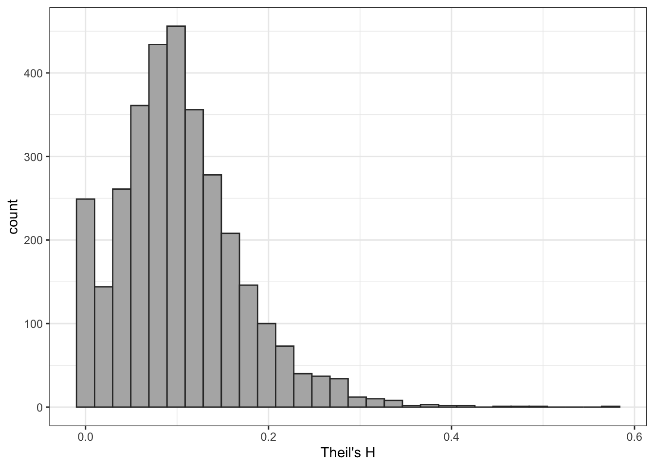
This is too many values to display, so lets go ahead and look at a histogram of Theil’s H across counties in the US:
ggplot(theil_h, aes(x = theil_h))+geom_histogram(color ="grey20", fill ="grey70")+theme_bw()+labs(x ="Theil's H")
Figure 13.1: Distribution of Theil’s H across US counties.
Mapping
For loops are fairly intuitive but have a bad reputation in R. Historically, for loops in R have been much slower than in many other programming languages (for reasons are that are technically complex). For that reason, many people prefer to use the methods of mapping rather than looping in R for speedier results. In more recent version of R, looping has improved considerably and so the advantages of mapping may be somewhat overstated. Nonetheless, it is useful to know both methods as mapping can sometimes offer other efficiencies over looping, or provide more compact code.
Our primary tool is going to be the map function from the purrr package. However, you can also use the lapply function from base R in the same manner. Both functions allow you to apply some other function to every element of a list.
Whats a list, you say? You may want to Chapter 3, but the short answer is that lists are collections of objects. The objects within lists can be of different types, but for the purposes of map and lapply we want lists that contain objects of the same type, since we are going to apply the same function to each element of the list.
The first step to getting map to work is to create the list. In our case, we want to split up our single dataset of all tracts to a list of datasets where each county is a separate element of the list. Each dataset within the list will have the same structure.
To split a dataset into a list of datasets, we can use the group_by command to define what variable should be used to split the list (county name and id, in this case), followed by a group_split command. For expository purposes, rather than splitting the full tract dataset, I am going to use the sample of ten counties from above.
The first element is the dataset for Alger County, Michigan. Each of the ten elements contains a dataset for a given county.
Now that I have my data structured the way that map wants the input, I can use the map function itself. The other required argument for map is a function that will be applied to each element of the list. I can use a pre-defined function or I can create a custom function. I will first demonstrate how it works by getting a summary for each dataset:
map(county_list, summary)
[[1]]
    tract_id         county_id     county_name          pop_total
 Min.   :2.6e+10   Min.   :26003   Length:3           Min.   :2203
 1st Qu.:2.6e+10   1st Qu.:26003   Class :character   1st Qu.:2696
 Median :2.6e+10   Median :26003   Mode  :character   Median :3190
 Mean   :2.6e+10   Mean   :26003                      Mean   :2955
 3rd Qu.:2.6e+10   3rd Qu.:26003                      3rd Qu.:3332
 Max.   :2.6e+10   Max.   :26003                      Max.   :3473
 pop_race_white pop_race_black  pop_race_asian  pop_race_other pop_race_multi
 Min.   :1925   Min.   :  2.0   Min.   : 2.00   Min.   :0      Min.   : 79
 1st Qu.:2126   1st Qu.: 10.0   1st Qu.: 2.00   1st Qu.:0      1st Qu.: 91
 Median :2328   Median : 18.0   Median : 2.00   Median :0      Median :103
 Mean   :2422   Mean   :230.3   Mean   :23.33   Mean   :2      Mean   :125
 3rd Qu.:2670   3rd Qu.:344.5   3rd Qu.:34.00   3rd Qu.:3      3rd Qu.:148
 Max.   :3013   Max.   :671.0   Max.   :66.00   Max.   :6      Max.   :193
 pop_race_latino  pop_race_indigenous
 Min.   : 28.00   Min.   : 18.00
 1st Qu.: 34.50   1st Qu.: 30.50
 Median : 41.00   Median : 43.00
 Mean   : 58.33   Mean   : 94.33
 3rd Qu.: 73.50   3rd Qu.:132.50
 Max.   :106.00   Max.   :222.00

[[2]]
    tract_id           county_id     county_name          pop_total
 Min.   :2.203e+10   Min.   :22025   Length:3           Min.   :1575
 1st Qu.:2.203e+10   1st Qu.:22025   Class :character   1st Qu.:2122
 Median :2.203e+10   Median :22025   Mode  :character   Median :2670
 Mean   :2.203e+10   Mean   :22025                      Mean   :2965
 3rd Qu.:2.203e+10   3rd Qu.:22025                      3rd Qu.:3660
 Max.   :2.203e+10   Max.   :22025                      Max.   :4650
 pop_race_white pop_race_black   pop_race_asian  pop_race_other pop_race_multi
 Min.   : 509   Min.   : 448.0   Min.   :0.000   Min.   :0      Min.   : 0.00
 1st Qu.:1362   1st Qu.: 739.0   1st Qu.:0.000   1st Qu.:0      1st Qu.:14.50
 Median :2215   Median :1030.0   Median :0.000   Median :0      Median :29.00
 Mean   :1962   Mean   : 935.3   Mean   :2.333   Mean   :0      Mean   :29.67
 3rd Qu.:2688   3rd Qu.:1179.0   3rd Qu.:3.500   3rd Qu.:0      3rd Qu.:44.50
 Max.   :3162   Max.   :1328.0   Max.   :7.000   Max.   :0      Max.   :60.00
 pop_race_latino pop_race_indigenous
 Min.   : 0.00   Min.   : 0.000
 1st Qu.: 3.50   1st Qu.: 0.000
 Median : 7.00   Median : 0.000
 Mean   :32.33   Mean   : 3.333
 3rd Qu.:48.50   3rd Qu.: 5.000
 Max.   :90.00   Max.   :10.000

[[3]]
    tract_id           county_id     county_name          pop_total
 Min.   :3.104e+10   Min.   :31043   Length:5           Min.   :2899
 1st Qu.:3.104e+10   1st Qu.:31043   Class :character   1st Qu.:3117
 Median :3.104e+10   Median :31043   Mode  :character   Median :3928
 Mean   :3.104e+10   Mean   :31043                      Mean   :4262
 3rd Qu.:3.104e+10   3rd Qu.:31043                      3rd Qu.:4535
 Max.   :3.104e+10   Max.   :31043                      Max.   :6829
 pop_race_white pop_race_black  pop_race_asian pop_race_other pop_race_multi
 Min.   : 879   Min.   :  9.0   Min.   : 63    Min.   :0      Min.   : 52.0
 1st Qu.:1037   1st Qu.: 15.0   1st Qu.: 63    1st Qu.:0      1st Qu.: 76.0
 Median :2430   Median :160.0   Median : 79    Median :0      Median : 85.0
 Mean   :1919   Mean   :299.2   Mean   :136    Mean   :0      Mean   :119.4
 3rd Qu.:2514   3rd Qu.:593.0   3rd Qu.:214    3rd Qu.:0      3rd Qu.:148.0
 Max.   :2737   Max.   :719.0   Max.   :261    Max.   :0      Max.   :236.0
 pop_race_latino pop_race_indigenous
 Min.   : 151    Min.   :  0.0
 1st Qu.: 970    1st Qu.: 24.0
 Median :1710    Median : 40.0
 Mean   :1696    Mean   : 91.4
 3rd Qu.:1872    3rd Qu.: 83.0
 Max.   :3778    Max.   :310.0

[[4]]
    tract_id          county_id     county_name          pop_total
 Min.   :2.91e+10   Min.   :29095   Length:224         Min.   :  23
 1st Qu.:2.91e+10   1st Qu.:29095   Class :character   1st Qu.:2051
 Median :2.91e+10   Median :29095   Mode  :character   Median :3042
 Mean   :2.91e+10   Mean   :29095                      Mean   :3194
 3rd Qu.:2.91e+10   3rd Qu.:29095                      3rd Qu.:3948
 Max.   :2.91e+10   Max.   :29095                      Max.   :7356
 pop_race_white   pop_race_black   pop_race_asian   pop_race_other
 Min.   :   6.0   Min.   :   0.0   Min.   :  0.00   Min.   :  0.00
 1st Qu.: 866.2   1st Qu.: 169.8   1st Qu.:  0.00   1st Qu.:  0.00
 Median :1702.5   Median : 507.5   Median : 29.00   Median :  0.00
 Mean   :1952.6   Mean   : 723.0   Mean   : 55.53   Mean   : 16.65
 3rd Qu.:2757.2   3rd Qu.:1051.5   3rd Qu.: 82.25   3rd Qu.: 11.00
 Max.   :5710.0   Max.   :3364.0   Max.   :421.00   Max.   :316.00
 pop_race_multi   pop_race_latino  pop_race_indigenous
 Min.   :  0.00   Min.   :   0.0   Min.   :  0.00
 1st Qu.: 58.75   1st Qu.:  90.5   1st Qu.:  0.00
 Median :103.00   Median : 183.5   Median :  0.00
 Mean   :126.01   Mean   : 306.1   Mean   : 14.39
 3rd Qu.:166.00   3rd Qu.: 346.2   3rd Qu.: 13.00
 Max.   :683.00   Max.   :2737.0   Max.   :403.00

[[5]]
    tract_id          county_id     county_name          pop_total
 Min.   :3.71e+10   Min.   :37103   Length:3           Min.   :2776
 1st Qu.:3.71e+10   1st Qu.:37103   Class :character   1st Qu.:2930
 Median :3.71e+10   Median :37103   Mode  :character   Median :3083
 Mean   :3.71e+10   Mean   :37103                      Mean   :3088
 3rd Qu.:3.71e+10   3rd Qu.:37103                      3rd Qu.:3244
 Max.   :3.71e+10   Max.   :37103                      Max.   :3404
 pop_race_white pop_race_black   pop_race_asian  pop_race_other
 Min.   :1727   Min.   : 642.0   Min.   : 4.00   Min.   :0
 1st Qu.:1854   1st Qu.: 712.0   1st Qu.:20.50   1st Qu.:0
 Median :1981   Median : 782.0   Median :37.00   Median :0
 Mean   :1913   Mean   : 854.7   Mean   :31.67   Mean   :0
 3rd Qu.:2006   3rd Qu.: 961.0   3rd Qu.:45.50   3rd Qu.:0
 Max.   :2031   Max.   :1140.0   Max.   :54.00   Max.   :0
 pop_race_multi   pop_race_latino pop_race_indigenous
 Min.   : 19.00   Min.   : 86.0   Min.   : 9.00
 1st Qu.: 53.50   1st Qu.:144.0   1st Qu.:18.00
 Median : 88.00   Median :202.0   Median :27.00
 Mean   : 90.33   Mean   :176.3   Mean   :21.67
 3rd Qu.:126.00   3rd Qu.:221.5   3rd Qu.:28.00
 Max.   :164.00   Max.   :241.0   Max.   :29.00

[[6]]
    tract_id           county_id     county_name          pop_total
 Min.   :5.506e+10   Min.   :55061   Length:5           Min.   :2370
 1st Qu.:5.506e+10   1st Qu.:55061   Class :character   1st Qu.:3260
 Median :5.506e+10   Median :55061   Mode  :character   Median :3724
 Mean   :5.506e+10   Mean   :55061                      Mean   :4114
 3rd Qu.:5.506e+10   3rd Qu.:55061                      3rd Qu.:5212
 Max.   :5.506e+10   Max.   :55061                      Max.   :6004
 pop_race_white pop_race_black pop_race_asian pop_race_other pop_race_multi
 Min.   :2208   Min.   : 0.0   Min.   : 0     Min.   : 0     Min.   : 37.0
 1st Qu.:2959   1st Qu.: 0.0   1st Qu.: 6     1st Qu.: 0     1st Qu.: 48.0
 Median :3522   Median : 3.0   Median : 6     Median : 2     Median : 68.0
 Mean   :3848   Mean   :19.4   Mean   :15     Mean   : 9     Mean   : 75.2
 3rd Qu.:4725   3rd Qu.:16.0   3rd Qu.:20     3rd Qu.: 4     3rd Qu.: 85.0
 Max.   :5827   Max.   :78.0   Max.   :43     Max.   :39     Max.   :138.0
 pop_race_latino pop_race_indigenous
 Min.   : 46     Min.   : 0.0
 1st Qu.: 81     1st Qu.: 0.0
 Median :100     Median : 0.0
 Mean   :139     Mean   : 8.2
 3rd Qu.:143     3rd Qu.: 5.0
 Max.   :325     Max.   :36.0

[[7]]
    tract_id           county_id     county_name          pop_total
 Min.   :2.809e+10   Min.   :28093   Length:10          Min.   :2164
 1st Qu.:2.809e+10   1st Qu.:28093   Class :character   1st Qu.:2742
 Median :2.809e+10   Median :28093   Mode  :character   Median :3594
 Mean   :2.809e+10   Mean   :28093                      Mean   :3398
 3rd Qu.:2.809e+10   3rd Qu.:28093                      3rd Qu.:3860
 Max.   :2.809e+10   Max.   :28093                      Max.   :4617
 pop_race_white   pop_race_black pop_race_asian pop_race_other pop_race_multi
 Min.   : 375.0   Min.   : 558   Min.   : 0     Min.   : 0.0   Min.   :  0.00
 1st Qu.: 998.2   1st Qu.: 918   1st Qu.: 0     1st Qu.: 0.0   1st Qu.: 27.75
 Median :1613.5   Median :1258   Median : 0     Median : 0.0   Median : 91.50
 Mean   :1600.6   Mean   :1548   Mean   : 4     Mean   :16.7   Mean   : 82.60
 3rd Qu.:2111.8   3rd Qu.:1989   3rd Qu.: 0     3rd Qu.:21.0   3rd Qu.:113.75
 Max.   :3098.0   Max.   :3470   Max.   :30     Max.   :99.0   Max.   :165.00
 pop_race_latino  pop_race_indigenous
 Min.   :  0.00   Min.   : 0.0
 1st Qu.: 27.75   1st Qu.: 0.0
 Median :112.50   Median : 0.0
 Mean   :145.20   Mean   : 1.4
 3rd Qu.:183.00   3rd Qu.: 0.0
 Max.   :477.00   Max.   :11.0

[[8]]
    tract_id           county_id     county_name          pop_total
 Min.   :3.607e+10   Min.   :36071   Length:92          Min.   : 1568
 1st Qu.:3.607e+10   1st Qu.:36071   Class :character   1st Qu.: 3327
 Median :3.607e+10   Median :36071   Mode  :character   Median : 4348
 Mean   :3.607e+10   Mean   :36071                      Mean   : 4361
 3rd Qu.:3.607e+10   3rd Qu.:36071                      3rd Qu.: 5130
 Max.   :3.607e+10   Max.   :36071                      Max.   :10758
 pop_race_white  pop_race_black   pop_race_asian   pop_race_other
 Min.   :  246   Min.   :   0.0   Min.   :  0.00   Min.   :  0.00
 1st Qu.: 1858   1st Qu.: 118.0   1st Qu.: 24.25   1st Qu.:  0.00
 Median : 2556   Median : 371.5   Median : 60.50   Median :  5.50
 Mean   : 2637   Mean   : 455.9   Mean   :123.46   Mean   : 21.59
 3rd Qu.: 3354   3rd Qu.: 623.5   3rd Qu.:180.50   3rd Qu.: 32.50
 Max.   :10080   Max.   :2405.0   Max.   :591.00   Max.   :256.00
 pop_race_multi  pop_race_latino  pop_race_indigenous
 Min.   :  0.0   Min.   :   0.0   Min.   : 0.000
 1st Qu.: 60.0   1st Qu.: 524.0   1st Qu.: 0.000
 Median :121.0   Median : 892.5   Median : 0.000
 Mean   :144.5   Mean   : 972.8   Mean   : 5.663
 3rd Qu.:186.8   3rd Qu.:1320.0   3rd Qu.: 0.000
 Max.   :618.0   Max.   :3221.0   Max.   :76.000

[[9]]
    tract_id           county_id     county_name          pop_total
 Min.   :5.115e+10   Min.   :51147   Length:6           Min.   :3124
 1st Qu.:5.115e+10   1st Qu.:51147   Class :character   1st Qu.:3178
 Median :5.115e+10   Median :51147   Mode  :character   Median :3394
 Mean   :5.115e+10   Mean   :51147                      Mean   :3654
 3rd Qu.:5.115e+10   3rd Qu.:51147                      3rd Qu.:3488
 Max.   :5.115e+10   Max.   :51147                      Max.   :5385
 pop_race_white pop_race_black pop_race_asian   pop_race_other
 Min.   :1636   Min.   : 702   Min.   :  0.00   Min.   : 0.000
 1st Qu.:1770   1st Qu.: 827   1st Qu.: 27.25   1st Qu.: 0.000
 Median :1966   Median :1152   Median : 29.50   Median : 0.000
 Mean   :2212   Mean   :1087   Mean   : 51.33   Mean   : 1.833
 3rd Qu.:2394   3rd Qu.:1286   3rd Qu.: 68.50   3rd Qu.: 0.000
 Max.   :3461   Max.   :1466   Max.   :141.00   Max.   :11.000
 pop_race_multi   pop_race_latino pop_race_indigenous
 Min.   :  0.00   Min.   : 46.0   Min.   :  0.00
 1st Qu.: 65.25   1st Qu.: 60.5   1st Qu.:  7.50
 Median :113.00   Median : 97.0   Median : 23.50
 Mean   :125.83   Mean   :131.8   Mean   : 44.33
 3rd Qu.:157.00   3rd Qu.:125.2   3rd Qu.: 29.75
 Max.   :308.00   Max.   :368.0   Max.   :185.00

[[10]]
    tract_id           county_id     county_name          pop_total
 Min.   :4.717e+10   Min.   :47167   Length:13          Min.   : 1566
 1st Qu.:4.717e+10   1st Qu.:47167   Class :character   1st Qu.: 2783
 Median :4.717e+10   Median :47167   Mode  :character   Median : 4849
 Mean   :4.717e+10   Mean   :47167                      Mean   : 4701
 3rd Qu.:4.717e+10   3rd Qu.:47167                      3rd Qu.: 5602
 Max.   :4.717e+10   Max.   :47167                      Max.   :10769
 pop_race_white pop_race_black   pop_race_asian   pop_race_other
 Min.   :1114   Min.   :  55.0   Min.   :  0.00   Min.   :  0.00
 1st Qu.:2028   1st Qu.: 286.0   1st Qu.:  0.00   1st Qu.:  0.00
 Median :2983   Median : 520.0   Median :  4.00   Median :  0.00
 Mean   :3504   Mean   : 869.5   Mean   : 26.23   Mean   : 31.31
 3rd Qu.:4603   3rd Qu.:1237.0   3rd Qu.: 26.00   3rd Qu.: 16.00
 Max.   :8682   Max.   :2938.0   Max.   :120.00   Max.   :169.00
 pop_race_multi  pop_race_latino pop_race_indigenous
 Min.   : 32.0   Min.   :  0.0   Min.   : 0.000
 1st Qu.: 70.0   1st Qu.: 35.0   1st Qu.: 0.000
 Median : 94.0   Median : 96.0   Median : 0.000
 Mean   :127.7   Mean   :138.2   Mean   : 4.154
 3rd Qu.:150.0   3rd Qu.:161.0   3rd Qu.: 2.000
 Max.   :445.0   Max.   :454.0   Max.   :26.000
This is a lot of information! By default, map returns a list of the same dimension as the input (in this case, 10 elements). In some cases, we can simplify this output, but not in this case.
Lets try creating a custom function within map itself. In this case, I want to get the sum of pop_total within each dataset.
In this case, I am actually writing the code for a custom function within another function. In this case, my function is quite simple, but you can use this feature to do some quite complex stuff if you want.
Again, the output is formatted as a list. However, I am returning a simple number for each value, so I would prefer that this output just be displayed as a simple vector of results. You can do this by using a variety of map_* functions where the second part indicates the return type you expect. In this case, I can use map_dbl because I expect the output to be a numeric value.2 Lets try it:
That seemed to work perfectly and gives me the same output as the for loop above. However, I would also like to get the county information returned in a table format. How, can I do that? I can use a custom function to output a tibble that includes the county name and id in the result:
[[1]]
# A tibble: 1 × 3
  county_name            county_id theil_h
  <chr>                      <dbl>   <dbl>
1 Alger County, Michigan     26003   0.136

[[2]]
# A tibble: 1 × 3
  county_name                 county_id theil_h
  <chr>                           <dbl>   <dbl>
1 Catahoula Parish, Louisiana     22025  0.0982

[[3]]
# A tibble: 1 × 3
  county_name             county_id theil_h
  <chr>                       <dbl>   <dbl>
1 Dakota County, Nebraska     31043   0.136

[[4]]
# A tibble: 1 × 3
  county_name              county_id theil_h
  <chr>                        <dbl>   <dbl>
1 Jackson County, Missouri     29095   0.228

[[5]]
# A tibble: 1 × 3
  county_name                  county_id theil_h
  <chr>                            <dbl>   <dbl>
1 Jones County, North Carolina     37103  0.0213

[[6]]
# A tibble: 1 × 3
  county_name                county_id theil_h
  <chr>                          <dbl>   <dbl>
1 Kewaunee County, Wisconsin     55061  0.0663

[[7]]
# A tibble: 1 × 3
  county_name                  county_id theil_h
  <chr>                            <dbl>   <dbl>
1 Marshall County, Mississippi     28093   0.143

[[8]]
# A tibble: 1 × 3
  county_name             county_id theil_h
  <chr>                       <dbl>   <dbl>
1 Orange County, New York     36071   0.145

[[9]]
# A tibble: 1 × 3
  county_name                    county_id theil_h
  <chr>                              <dbl>   <dbl>
1 Prince Edward County, Virginia     51147  0.0493

[[10]]
# A tibble: 1 × 3
  county_name              county_id theil_h
  <chr>                        <dbl>   <dbl>
1 Tipton County, Tennessee     47167   0.129
This approach worked, but because I am returning a tibble each time, I am back to the list format for my output. What I want is each of these results as rows of a shared tibble. Luckily, bind_rows will do this for me. I just have to pipe the results of map into a bind_rows to get everything formatted nicely:
# A tibble: 10 × 3
   county_name                    county_id theil_h
   <chr>                              <dbl>   <dbl>
 1 Alger County, Michigan             26003  0.136
 2 Catahoula Parish, Louisiana        22025  0.0982
 3 Dakota County, Nebraska            31043  0.136
 4 Jackson County, Missouri           29095  0.228
 5 Jones County, North Carolina       37103  0.0213
 6 Kewaunee County, Wisconsin         55061  0.0663
 7 Marshall County, Mississippi       28093  0.143
 8 Orange County, New York            36071  0.145
 9 Prince Edward County, Virginia     51147  0.0493
10 Tipton County, Tennessee           47167  0.129
Now the format is working perfectly. Lets go ahead and apply this to the full dataset in one pipe:
# A tibble: 3,222 × 3
   county_name                      county_id theil_h
   <chr>                                <dbl>   <dbl>
 1 Abbeville County, South Carolina     45001  0.127
 2 Acadia Parish, Louisiana             22001  0.263
 3 Accomack County, Virginia            51001  0.129
 4 Ada County, Idaho                    16001  0.110
 5 Adair County, Iowa                   19001  0.0902
 6 Adair County, Kentucky               21001  0.0768
 7 Adair County, Missouri               29001  0.0843
 8 Adair County, Oklahoma               40001  0.0424
 9 Adams County, Colorado                8001  0.122
10 Adams County, Idaho                  16003  0.0240
# ℹ 3,212 more rows
Students often go with the for loop approach because it feels more natural and intuitive. In particular, students are often scared off by the custom function business. However, mapping offers you more flexibility and often speed, and so its worth learning. In this case, it was much easier to get both county name and id in the final output using mapping rather than looping.
We can also wrap each command in system.time to see how they actually perform in terms of time.
theil_h <-NULLsystem.time(for(county in counties) {# calculate Theil's H for this county h <- tracts |>filter(county_name == county) |>calc_theil_h()# add this county's values to our dataset of values theil_h <- theil_h |>bind_rows(tibble(county_name = county, theil_h = h)) })
The difference in speed is pretty minimal here. The for loop takes about 10% more time, which amounts to 2 seconds in this case. For many operations, this gain is probably not enough to warrant a decision on looping vs. mapping. However, for computationally intensive operations, a 10% savings in time may make a big difference in absolute time.
The other option is a while loop which will repeat the same code until a condition is met.↩︎
The equivalent approach to lapply is to use sapply which simplifies the list to a vector if possible.↩︎